Torticollis is a condition where an infant's neck muscle is tight or shortened on one side, causing the head to tilt in one direction. Congenital muscular torticollis (CMT) is the most common form and is typically identified in the first few months of life. Physical therapy with gentle stretching, positioning strategies, and parent education is the primary treatment.

Do you accept TRICARE?

Yes. Lead Pediatric Physical Therapy is an in-network provider with TriWest Health Care Alliance, which administers TRICARE West. Your provider can call 844-866-9378 to enter a referral. We are honored to serve military families in Fort Worth.

Do you offer in-home physical therapy visits?

Yes. In-home and daycare visits are available within a 15-minute drive of our clinic in the 76107 area of Fort Worth. Your child receives the same one-on-one care with Chrissy in the comfort of their own environment.

What is a PCS certification?

PCS stands for Pediatric Clinical Specialist, a board certification awarded by the American Board of Physical Therapy Specialties. Fewer than 3 percent of physical therapists in the United States hold this credential. It requires advanced clinical experience and a rigorous examination focused exclusively on pediatric physical therapy.

How much does a pediatric physical therapy evaluation cost?

The initial evaluation is $185 and lasts 45 to 60 minutes. Follow-up one-hour treatment sessions are $155 and half-hour sessions are $95. Packages are available at a reduced rate. We accept HSA and FSA cards, credit and debit cards, and Venmo.

What should I bring to my child's first physical therapy appointment?

Bring any referral paperwork from your pediatrician, a list of your concerns and questions, and your child in comfortable clothing. If your child is an infant, bring a favorite toy or comfort item. Chrissy will spend time understanding your child's history and your goals before beginning the evaluation.

Posts by:

Tim Booher

Engineering & Code

Understanding and Fixing my Gate

Texas introduced us to cowboy hats and electric gates, in our case a a Nice Apollo 1500LA. It’s a long-running linear actuator swing gate: simple enough to be something I can repair, but just complicated enough to be difficult. The whole gate is really two different parts: a 636 control board and a 816 actuator. In the past, I documented how I connected our gate to Alexa through a WiFi connection in Gate Automation. This post is about how our gate works and how to fix it.

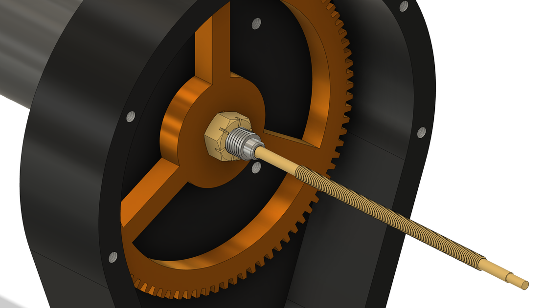
Our gate started opening past the limit switch and now I have to fix the 816 actuator, it’s a 12-volt DC motor that turns a pinon and spur gear which drives the central Acme lead screw. I had just fixed the broken spur gear and the old motor that lost much of its usable torque under load. After a couple of successful months after I replaced the motor and the spur gear, the limit screw broke and the gate only stopped at at absolute min extension. Slide below to see all these parts and how they work.

Illustration 1 – Drag the slider to open the housing and run the gears.

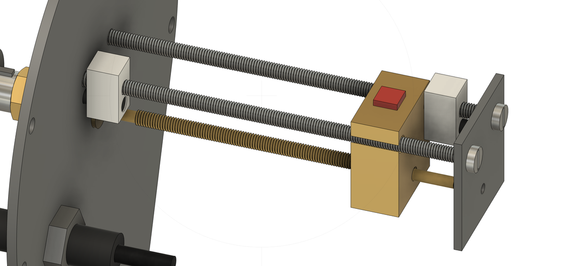
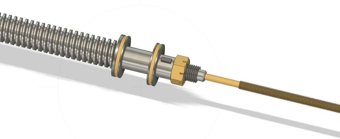
I opened up the housing to find that the A2019 limit screwwas broken and the key was broken as well. The A2019 limit screw threads directly the end of theACME lead screw so they move together. The illustration below shows how this works. A travellercarrying amagnetrides on the limit screw‘s thread. Two guide bolts keep the magnet from turning.

Illustration 2 – The traveller walks along the A2019 limit screw until a switch trips.

As the arm extends or retracts, the traveller walks slowly along the tower. Its position mirrors the gate. At each end of its travel sits a proximity switch on a limit block. When the magnet reaches a switch, the switch trips and tells the control board to stop the motor, one switch for fully open and one for fully closed.

**Fig** 1 – The traveler uses the guide bolts to stay vertical

So how does a magnet generate a signal to the controller board? A magnet induces an electric field. As the magnet approaches, the field strength $B$ at the switch climbs steeply, roughly as $1/d^3$, but continuously. My guess is that the gate has a Hall-effect sensor where current through a thin semiconductor is pushed sideways by the field, producing a tiny voltage proportional to $B$. On its own that’s still analogue. An on-chip Schmitt trigger (a comparator with two thresholds, on above one and off below a lower one) flips its output transistor fully on or off.

Another interesting thing: the lead screw moves about 5 tpi (threads per inch) or 0.20–0.22 $in$ per turn to fully open the gate, but the limit screw moves about $ \frac{1}{8}^{\text{th}} $ that distance. In all, whole 2 ft of arm travel is shrunk into about 3 in of traveller movement. Simply, the screw goes a distance $L$ which is each spiral thread winding around the screw $n_{\text{starts}}$ $\times$ the pitch $p$ of each screw.

L = n_{\text{starts}} \cdot p = \frac{n_{\text{starts}}}{\text{TPI}}

In this setup, both screws turn together. The limit screw is fixed to the end of the lead screw, so after a common set of $ N$ revolutions each screw goes a total length $s$ of:

s_{\text{arm}} = N \cdot L_{\text{lead}} \qquad s_{\text{trav}} = N \cdot L_{\text{limit}}

For the full stroke the revolutions are the same,

N = \frac{24\;\text{in}}{0.21\;\text{in/rev}} \approx 114\ \text{rev}

\, L_{\text{Lim}} = \frac{s_{\text{trav}}}{N} = \frac{3.6 \, \text{in}}{144\, \text{rev}} = 0.025 \,\text{in/rev} = 40 \, \text{tpi}

So the lead screw has 8x the thread density and goes 8x shorter in length.

**Fig** 2 – Lead screw versus limit screw threads

The geometry of the setup can teach us a lot about how stuff works. The lead screw pushes the rod out several feet, but it pushes only about 4.5 ft from the hinge, so a short push near the pivot becomes a long sweep at the gate’s far end. Two feet becomes 25 feet: about 20 in of stroke swings a 16 ft gate through 90°, and its tip travels about 25 ft, a quarter of a 100 ft circle. That is about 15× multiplication: the actuator’s average lever arm is about 12.7 in, compared with the tip’s 192 in, so each inch of push moves the tip about 15 in.

But nothing comes for free. The trade-off is force: holding the gate against a push at its tip takes about 15 times that force at the rod, which is why the motor’s torque is multiplied first by the gears and the ACME screw. All together, the whole chain: about 840 motor turns leads to 114 screw turns leads to 24 in of arm travel which is about 25 ft at the gate tip.

The most interesting thing for me is the offset arm. Without it the lead screw would just pull on the hinge and not push out. The bigger the offset arm, the more force transfers to the tip of the gate. How big should we make this offset? The manual recommends 6 $\text{in}$ which has enough lever arm to break the gate away from closed, while keeping the stroke inside the actuator. More offset means a longer stroke for 90°. The actuator swings through a bigger angle, and past a point it runs out of its 24 in, which is the demo’s warning.

Arm offset	Lever arm at start	Hinge torque	Force at tip
0 in	0 in	0 lb·ft	0 lbf (stuck)
2 in	≈ 2.5 in	≈ 73 lb·ft	≈ 4.6 lbf
4 in	≈ 5.0 in	≈ 146 lb·ft	≈ 9 lbf
6 in (manual)	≈ 7.5 in	≈ 219 lb·ft	≈ 14 lbf
9 in	≈ 11.4 in	≈ 333 lb·ft	≈ 21 lbf

The experiment below brings all this together. Move out the pivot arm to see the effect on the force.

Illustration 3 – Change the pivot arm and drive, then open the gate.

Now that we know how everything works, I actually have to fix this gate and put the washers and spur gear together.

**Fig 3** – The spur gear and screws form a rigid system

The washers in the A2087 include two needle thrust bearings. Every time the actuator pushes or pulls the gate, the gate pushes back along the lead screw, trying to shove the whole screw lengthwise out of the housing with hundreds of pounds of force. A thrust bearing takes that end-to-end load while still letting the screw spin freely. Each bearing is a sandwich. In the middle is a flat steel cage holding about twenty tiny hardened needle rollers, arranged like the spokes of a wheel. On either side is a hardened, polished race: the thin washers, plus one thicker race for the screw’s shoulder. The needles roll between the races instead of sliding, so the friction stays low even under heavy load. The races matter as much as the rollers, because they give the needles a hard, smooth track; without them, the needles would quickly dig grooves into the softer housing and gear. When a gate is making bad sounds opening and closing, it’s generally overlooked parts like this.

**Fig 4** – Nice Apollo Bearing Kit (A2087)

The biggest problem for me is that little piece on the bottom right. Known a key, it’s the smallest part that does the most work: ensuring the torque is transfered from the rotating shaft to the spur gear which sits on a round, smooth section of the shaft. On its own it would just spin in place, or slip under load. To make this work, a small slot is milled lengthwise into the shaft (the keyseat), and a matching slot runs through the gear’s bore (the keyway). The square key sits half in each, bridging the two parts. All of the motor’s torque passes through that little 3/32 $\text{in}$ bar. The Flexloc nut only stops the gear sliding off the end; it isn’t what makes the gear drive the screw.

As an engineer, I look at parts like this carefully. The key is like the derailleur hanger on your bike, strong enough to work, but weaker than the expensive parts around it. If the gate jams hard, it tends to shear the cheap key, saving a costly stripped gear or a twisted screw.

The final experiment is the diagram that matters for my current fix. Explode the assembly to see how the key ties everything together.

Illustration 4 – Explode the stack; click any part to hide it.

Hopefully this post gave you new appreciation for the beauty and thought that goes into the simple stuff around you. Today the combination of AI, youtube and Amazon/e-commerce let you understand, learn and find any part you need. These are amazing days to be a builder.

September 28, 2026 (updated September 28, 2026) By Tim Booher 0 Comments

Engineering & Code

Digital Trees

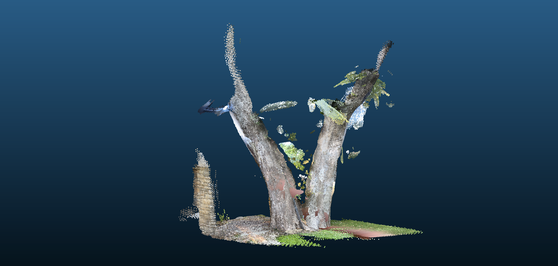
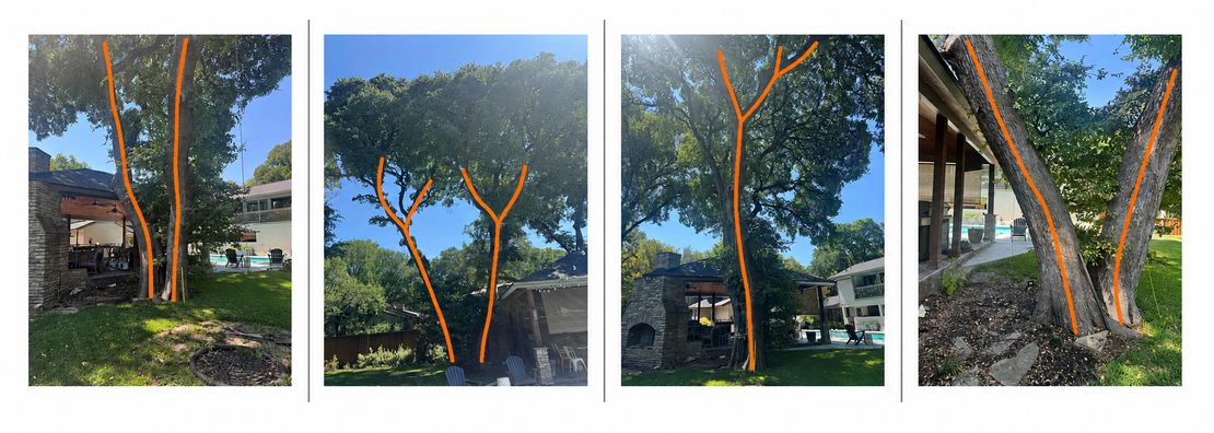
This tree is in my backyard, right behind our cabana. Go ahead, move it around and I’ll explain below how an iPhone + claude + plus some cool geometry math made this happen.

Loading tree…

I’ve always been fascinated by trees. I love how they grow in seemingly random ways, yet also obey a fixed set of rules. They form the backdrop of so many of my favorite places, always telling a story about the soil they are in and the geography around them.

In building a 3-D model of my house, I had to figure out some way to model the trees in my yard. Two things make a full model of a tree hard. First, it’s not feasible (and stupid) to get up 40 ft and do a laser scan of every branch. Second, a native scan would be huge and not useful in an architecture model.

This turns out to be a mixed-fidelity problem. You can build a mesh pretty easily, using an AI-powered tool like TRELLIS or Meshy to generate an actual mesh, resulting in hundreds of thousands of triangles without a lot of associated meaning. At the top of the tree, that may be perfectly fine. The canopy needs to be dimensionally correct and visually plausible, but the higher you go, the less it matters where each branch is located.

At the base of the tree, though, it matters a lot. A major split in the trunk, the direction of a large branch, or a limb extending over a building I’m working on can be important. The bottom of the tree needs to be real, while the top just needs to look right and be close to the correct height.

Ultimately, Revit and then rendering tools like Enscape or Trellis need the right fidelity, not maximum fidelity. And the most useful representation may not be a mesh at all. It may be a set of nodes, connections, dimensions, and rough geometry.

The ideal geometry is just a bunch of connected, tapered cylinders. Turns out someone has thought of this before the the internet is full of tree making programs. Enter Quantitative Structure Models, or QSMs. Instead of storing a tree as a giant triangle mesh, a QSM represents the trunk and branches as a connected graph of tapered cylinders: each segment has a start point, end point, radius, and parent-child relationship. That gives us exactly the right data structure for this problem because the measured lower part of the tree can remain geometrically accurate, while the unmeasured upper branches can be generated by Claude. This both looks accurate, but renders fast.

The iPhone and SiteScape can get me a good point cloud. No top of the tree, not even a mesh, just a bunch of dots and only observed at my height and below.

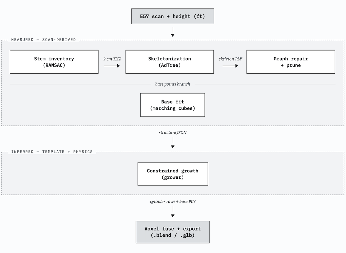
The approach that works is measurement-first, inference-last. A phone/terrestrial scan of a backyard tree only captures the lower 5–6 m, so the pipeline splits the problem: everything the scanner saw is reconstructed and locked, and everything above the scan ceiling is grown by a AI with a constraint engine rather than invented freehand.

To get this right we want to give Claude all the data with an open-source tool (AdTree) that automatically reconstructs a tree’s branch skeleton and geometry from a laser-scanned point cloud. The constraints are: species (cedar elm), no central leader, sympodial forking, scaffolds arching outward), a photo-derived crown envelope, a surveyed height (46 ft by yardstick and ChatGPT), pipe-model taper at every fork, and a tapered-cantilever beam check that rejects branches that couldn’t carry their own weight. The LLM’s job is proposing and tuning those constraints and deciding which branches matter, not drawing geometry.

Forestry research tools (TreeQSM, AdTree, TreeAIBox, 3DFin) are mature at turning point clouds into cylinder models, but they reconstruct everything for biomass estimation: thousands of cylinders, collapsing radii where the scan is sparse. They are awesome, and mostly built to reconstruct a forest. My architectural models need the opposite: a few hundred faces with believable structure. So the pipeline deliberately inserts a decimation step (keep scaffolds, drop twigs) and re-derives upper radii from the trustworthy dense-zone measurements instead of the QSM’s guesses. Everything below ran locally: the reconstruction chain on a Mac (AdTree built from source, Blender via MCP for geometry), with CloudCompare’s Windows build adding TreeIso, 3DFin and TreeAIBox as a second, independent QSM to cross-check the first.

The output is pretty cool. I get a real tree that is watertight, parametric, computationally simple and structurally similar to the actual tree.

AdTree (Tech Details)

I took a look under the hood to see how AdTree works. It’s pretty cool.

AdTree converts a single-tree point set $ P=\lbrace\mathbf{p}_{i}\rbrace_{i=1}^{N}\subset\mathbb{R}^{3}$ into a rooted skeletal graph rather than reconstructing a surface directly. It first identifies points likely to lie on major branches from locally stable point density and contracts them toward branch centerlines using mean-shift. It then constructs a 3-D Delaunay proximity graph $G_D=(V,E_D)$, assigns each edge the Euclidean cost $\ell_{ij}=\lVert\mathbf{p}_{i}-\mathbf{p}_{j}\rVert_{2}$, and applies Dijkstra’s algorithm from the tree base to form what the paper calls a minimum spanning tree—more precisely, a rooted single-source shortest-path tree embedded in the cloud. Each skeletal vertex receives an importance $W(v)=\sum_{e\in T_v}\ell_e$, defined as the total length of the edges in its descendant subtree, while each edge receives the mean importance of its two endpoints; low-importance basal artifacts are then pruned. Degree-two vertices are removed using a Douglas–Peucker-type test $\alpha=d/r\leq\sigma$, where $d$ is the vertex’s distance from the parent–child chord and $r$ is a local edge scale, implemented using the parent-edge radius. At bifurcations, two child vertices are eligible to be merged when $\alpha=\min\left(\ell_1\sin\theta/r_2,\ell_2\sin\theta/r_1\right)\leq\sigma$, with the replacement vertex positioned at $\mathbf{p}_{\mathrm{new}}=(W_1\mathbf{p}_1+W_2\mathbf{p}_2)/(W_1+W_2)$. In the source implementation, merging is additionally restricted to child edges separated by an angle of approximately $26^\circ $ or less and having lengths within a factor of two. This procedure repeatedly contracts redundant graph structure while attempting to preserve the tree’s major branching topology.

Geometry is then attached to the simplified skeleton by fitting generalized cylinders. Points near the well-sampled lower trunk are retrieved using a spatial or $k$-d-tree query. The trunk-cylinder parameters—an axis unit vector $\mathbf{a}$, a point $\mathbf{c}$ on the axis, and a radius $r$—are estimated by Levenberg–Marquardt minimization of the radial residual:

$$
e_i(\mathbf{a},\mathbf{c},r)= \left\lVert(\mathbf{p}_{i}-\mathbf{c})-\left[(\mathbf{p}_{i}-\mathbf{c})\cdot\mathbf{a}\right]\mathbf{a}\right\rVert_{2}-r,\qquad \min_{\mathbf{a},\mathbf{c},r}\sum_i e_i^2.
$$

AdTree then performs a second, robustified fit using $q_i=1-\lvert e_i\rvert/\max_j\lvert e_j\rvert$. In the source implementation, $q_i$ multiplies the residual passed to the least-squares solver, so the implemented objective is $\sum_i(q_i e_i)^2$, reducing the influence of distant outliers. Because crown points are generally too sparse and noisy for reliable independent cylinder fitting, the remaining edge radii are inferred allometrically from subtree importance. The paper states the linear relationship $r_e=r_t(W_e/W_t)$, where $r_t$ and $W_t$ belong to the fitted trunk; the source implementation instead uses $r_e=r_t(W_e/W_t)^{1.1}$. After skeleton smoothing, generalized cylinders with varying endpoint radii are constructed along the skeletal paths and triangulated into the final OBJ mesh. Leaves are synthesized near terminal branches rather than reconstructed from LiDAR. You can think of AdTree as a graph extraction + topology-preserving simplification + partial geometric fitting + allometric completion algorithm, not a neural or direct point-to-mesh method.

I had to take this and make a hybrid technique. First, I derive all parameters diameter at breast height (DBH) is fitted by RANSAC circle regression during stem inventory; the crown envelope, branching rules, and mechanical limits come from a species template scaled to the input height; and growth seed points are computed from the measured skeleton rather than authored by hand. A single orchestrator (maketree.py) executes the nine stages as subprocesses of the repository’s stage scripts, prints a per-stage status line with wall-clock time, and halts on any gate failure. On current hardware (Apple M-series) a five-million-point scan completes in roughly twelve minutes, of which the AdTree skeletonization stage accounts for approximately nine.

The design principle is measure where the scan is dense, infer where it is not, and let physics referee the boundary. Below 3.05 m (10 ft), where point density is highest, the trunk union is meshed directly from an occupancy grid by marching cubes, no cylinder abstraction at all, because a multi-stem base is a fluted solid that swept tubes cannot represent. Above that, AdTree’s skeleton is reduced to a canonical branch graph, repaired (single-rootedness, child-to-parent attachment gap ≤ 5 mm, cloud-support pruning of spurious stubs), and extended to the surveyed height by a constrained grower whose proposals must survive a tapered-cantilever beam check and a slenderness floor $ r ≥ L/90 $ before emission. The completed skeleton is exported in TreeQSM’s cylinder interchange format, deliberately reusing the Inverse Tampere Blender add-on rather than a bespoke mesher, and the tube crown and fitted base are fused by a single voxel remesh, which yields one watertight component and makes the seam, pinch, and open-cap defect classes structurally impossible rather than individually patched.

August 30, 2026 (updated August 31, 2026) By Tim Booher 0 Comments

Personal Projects & Interests

A hometown tragedy and the need for Grace

On September 29, 2026, Caleb Flynn, a former worship pastor and American Idol contestant, was convicted of murdering his wife, Ashley, a teacher, volleyball coach, and mother of two. Ashley was shot in their Tipp City, Ohio, home in February. Prosecutors presented evidence that Caleb, who was having an affair with a fellow worship leader, staged a burglary to conceal the killing.

This story is sad and disorienting. It’s sad because of the destroyed dreams, the broken promises and the glaring betrayal executed under the highly produced protection of evangelical Christianity. It’s disorienting because this is my small hometown. In high school, I preached a sermon to the Christian Life Center youth group. It’s a place I think about every time I land at Dayton airport. Ashley Flynn lived and was murdered right next to my high school. While I don’t think I met her, she was the 4th grade teacher and volley ball coach to friend’s kids. She was friends with several folks in my family.

But it’s more than that. It’s disorienting because the villains here are relatable as they are repulsive. On the surface, Caleb Flynn is wildly different than me. I have no real musical talent, exist in a different community of global engineering and technology, and am much less rooted nor known in my local hometown. I don’t sell furniture and he is ten years younger than me. Still, we are both husbands, fathers and connected to the same small part of the world that is the Christian community of north Dayton Ohio.

My theology tells me that I’m morally no better (nor worse) than Caleb Flynn. Any goodness I that I get to participate in is only a gift from my Creator. That said, a close friend told me, “But Tim, you didn’t have an affair and kill your wife.” He is right, and that difference matters. Faithfulness and betrayal are not morally equivalent. But the goodness of my choices does not make me the source of that goodness. God’s grace does more than forgive sin; it renews the heart, strengthens obedience and teaches us to love what is good. Whatever faithfulness He has worked in me is real, but it remains a gift. We Christians are responsible for our choices, yet dependent on Him for the strength to choose rightly.

One of the Bible’s greatest heroes was a man after God’s own heart. God gave King David the courage and strength to slay the giant who oppressed an entire nation. And yet, “he saw a woman bathing, and the woman was very beautiful to look at” (2 Samuel 11:2). That “beautiful” sight led him to send for her start an illicit affair. When she became pregnant, he tried to conceal what he had done and finally arranged the death of her husband, Uriah, a loyal and honorable man. Thousands of years apart, same pattern of brokenness and pain.

Arrogance, pride, lust, power universally tempt all of us, even when CS Lewis already excellently summed up how sin destroys joy in the banter between two demons: “An ever increasing craving for an ever diminishing pleasure is the formula.”¹

When we know where a path leads, why can its beginning still look so attractive? I find something uncomfortable in my own response to this story and the way media elevates the emotional parts of romance over commitment and duty. Alongside the disgust and sadness, I recognize the appeal of being intensely wanted, of novelty, of a secret that makes ordinary life feel suddenly electric. I can fully and completely understand the start of the road this man went down. We imagine enjoying the thrill while escaping the cost, as though the pleasure could be separated from the people we would betray. Knowing that a desire is destructive does not necessarily make us stop wanting it. We need grace not only to govern our actions, but to correctly order and change what we love.

But despite the public’s fascination with an illicit love story, Ashley’s death confronts us with a person betrayed and a family shattered. What looks like romance when we leave out those who suffer becomes truly evil when we bring them back into view.

Ashley Flynn was a woman whose profile picture consistently included her husband. Ashley knew her marriage was struggling, but she was fighting for it. In a note saved on her phone, she wrote, “We really need Jesus to intervene.” Later, her goals included getting on the same page with Caleb. Meanwhile, Caleb was sending his mistress messages saying he hated Ashley and wanted her dead. Her family had welcomed him into their lives and trusted him with a place in their business.

Here is a man with enumerable blessings. Nothing is more precious (and rare) in our modern world than having roots and meaning. Nothing is more sought after than to be the guy that other men want to be and who comes home to an adoring wife. His place in the community and christian affiliations led to success in his job selling furniture and flooring to churches. He had a beautiful wife and daughters who adored him. He had a wife fighting for their marriage until she was shot twice in the head. Damn.

What, if anything, does great blessing have to do with great sin? Ashley Flynn could still be dead from an unlucky bum who couldn’t carry a tune. We have this phrase “special place in hell” for sin that gets wrapped in special packaging, but I just can’t rev up the engine of injustice and anger for this situation. The destruction is raw in front of us as we watch this ghoul of a once alive man sit in the middle of a room while the system orchestrates the deserved destruction of his life.

He is simultaneously both present and absent in that courtroom. Absent because he can’t live like we can in the present, building things and hugging those we love. He appears to be only living in the regretful past and in a terrible future, helpless to do anything to change his situation. My faith tells me that there is always hope of redemption. King David experienced incredible loss and met it with true repentance and eventually restoration. That clearly isn’t possible without confession of some sort, so this man seems stuck, locked out of the present.

What is a good man to feel about all this? What should a good man want from where we are now? Extreme sadness for the loss? Gratefulness for the embrace of my own family? Comfort in the good reward of my better choices? Glad to watch the wheels of justice turn? All the above?

I want justice, but I find no satisfaction in the ruin before me. So it’s definitely sadness combined with fear of just what someone from my community is capable of. I resonate with all of those questions, but I don’t know how to hold them together except by running into my Father’s arms and thanking him for sparing me and the people I love a road like this. That leaves me in love with His goodness and thankful for every breath. At some point, thankfulness merges into worship.

And that’s an odd place to end up: worship . . . the very job of this once-among-us man named Caleb Flynn. A man who once with his mistress led a crowd of worshiping Christians. The picture tells us a truth: hands lifted up, the crowd was looking past that the two of them to a risen Savior who is still good and who knows what this all means. Here very fallen people have dishonored God’s name, but they (and we) cannot diminish His goodness or glory.

Caleb Flynn has destroyed his marriage, his own life and deeply wounded his family and his community. God remains good. I remain thankful. Come Lord Jesus.

C. S. Lewis, The Screwtape Letters, Letter IX (9) ↩︎

August 6, 2026 (updated October 2, 2026) By Tim Booher 0 Comments

Engineering & Code

Cyber Defense Is Losing

While at DARPA I once debated that Cybersecurity would at some point be solved. I argued that if we just built and implemented software correctly, DEFCON would be no more exciting than whatever the people who make bolts and hardware do for a convention. Boring, commoditized and expected.

Well, I’ll concede that cyber isn’t getting solved anytime soon. While AI may eventually present the ability to develop and implement secure software, right now the attacker is getting nearly all the benefits. This is because AI generated code is buggy, our world is increasing in scale and complexity, and now offense is easy while defending remains hard.

For a long time, there has been a fragile balance between offense and defense — a perfect environment to build a cyber company. Everything has been getting bigger and more digital at once: more data, more devices, more software, more dependencies. Complexity and scale make defense difficult, but new tech always rose to this challenge. This all worked as long as offense remained the domain of the skilled hacker.

Recent AI advances turn two known properties of the offense/defense game into a big problem at scale, tipping this balance. The life blood of cyber is vulnerability discovery, we learn how software can break. This information allows attackers to write exploits to take over systems, while defenders implement patches to fix the software.

First, while both are fragile, exploits are certain while patching is an exercise in hope. Once an attacker has working exploit code, it tends to work the same way every time against every still-vulnerable target. The attacker has a master key. The defender, by contrast, has to run a messy social and technical process: identify the affected systems, test the fix, schedule the outage, avoid breaking production, coordinate with vendors, and hope nothing critical was missed. You never really know how certain a patch is. The exploit (and the access it gives you) is truth. The patch is a potential improvement in security.

Second, offense needs one opening while defense needs universal coverage. A large enterprise is not defending a single castle wall. It is defending an every changing city with millions of doors: endpoints, cloud workloads, identities, APIs, SaaS integrations, vendor pathways, forgotten development environments, and software libraries nested inside software libraries. The attacker only needs one of those doors to stay open long enough to matter.

Those two facts explain more about the current cyber moment than most product categories, frameworks, or buzzwords. And both of them are radically accelerated by the long trend that mythos is putting right in front of us.

The Patch Gap

Think of a flaw in a widely used lock. The moment someone publishes a working bypass, every copy of that lock in the world shares the same weakness. The offensive advantage arrives instantly and spreads perfectly. The defensive fix does not.

That fix has to diffuse through institutions. Some teams patch in hours. Some patch in weeks. Some wait for a vendor. Some do not know they are exposed. Some know, but cannot patch without risking a more immediate outage. Some are carrying vulnerable code inside a container inside a product they do not control. The result is the same pattern every time: attacker capability jumps to near total coverage immediately, while defender coverage crawls upward over months or years and never quite reaches 100 percent. Additionally, the patch will prevent the known mechanism of the exploit, but do other vulnerabilities exist? Maybe the new patch created them.

This is the patch gap. It is where a large fraction of real-world compromise lives.

Real example: Log4Shell made the pattern visible to everyone. The vulnerability was obvious, the exploitation path was clear, and the world still spent months chasing it. Years later, defenders were still seeing exploit attempts because the tail never fully disappeared. The lesson was not just that organizations should patch faster. It was that patching is constrained by logistics, testing, ownership, incentives, and plain institutional friction. Even when everyone agrees on what should happen, it does not happen uniformly.

AI makes this worse before it makes it better. It is already helping discover vulnerabilities faster, write proof-of-concept exploits faster, and scale reconnaissance faster. That compresses the time between flaw discovery and usable offensive tradecraft. Unless defensive remediation becomes equally automated, the patch gap widens.

One vs. All

The second asymmetry is simpler and harsher. Attackers need one success. Defenders need comprehensive performance across an enormous attack surface.

There is a reason experienced defenders sound pessimistic even when they are competent. They have internalized the arithmetic. If an organization has $n$ things that can fail, and each of them is secure with probability $p$ on a given day, then the chance that everything is secure is $p^n$. Once $n$ is large enough, even very high values of $p$ stop feeling reassuring.

That is not a slogan. It is a scaling law.

Suppose your controls are extremely good. Suppose each asset is secure 99.999 percent of the time. That sounds excellent until you apply it across millions of assets, identities, services, and dependencies. The question stops being whether a failure exists and becomes where it exists, how exposed it is, and whether the attacker finds it before you do.

This is why “we are pretty good on average” is not a comforting statement in cyber defense. Averages do not defend networks. Coverage does.

It also explains why the workforce problem is not simply a hiring problem. The surface being defended has grown much faster than the workforce available to defend it. Cloud expansion, SaaS sprawl, API dependency chains, machine identities, and AI-generated code have all increased the number of doors faster than institutions can add trained defenders. Even if every hiring pipeline worked better, the denominator is still outrunning the numerator.

Why AI Changes the Balance

AI does not create these asymmetries, but it does intensify them. The core question is “what can AI do and what permissions do we give it?” It can now exploit the software it’s given. It can (and should not) have access to all computers and the authority to quickly patch them.

On offense, AI lowers the cost of attacks that used to be too expensive to bother with. Tailored phishing, malware variation, vulnerability research, and exploitation support all become cheaper and faster. That means more attackers can attempt more operations against more targets. It also means one-off attacks against smaller or previously uninteresting targets become economically viable.

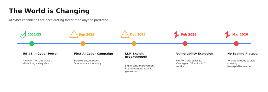
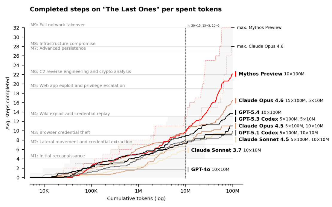
In April 2026, the UK AI Security Institute (AISI) published its evaluation of Claude Mythos Preview and reported that the model had, for the first time, completed a full 32-step corporate-network attack simulation end-to-end — from initial reconnaissance through full domain takeover — on a purpose-built cyber range. The scenario is estimated to take a human professional around twenty hours. Mythos Preview solved it start-to-finish in 3 of its 10 attempts and, across all attempts, completed an average of 22 of the 32 steps. On the expert-level individual tasks that no model could finish before April 2025, the same model succeeded 73 percent of the time. Two years earlier, frontier systems could barely complete beginner-level capture-the-flag challenges.

The chart below shows how far each frontier model gets through a multi-stage attack chain — from M1 (initial reconnaissance) up through M9 (full network takeover) — as compute budget grows. The headline is simple: Mythos is the only model that finishes the chain. Every other frontier model, including Claude Opus 4.6 and GPT-5.4, stalls somewhere in the middle — credential theft, lateral movement, infrastructure compromise — no matter how many tokens you give it. Mythos keeps going and takes over the network. There is no visible plateau in the trend, and the newest model is the one pushing autonomous exploitation from partial to end-to-end.

The Institute was careful about what this does and does not mean. The cyber ranges lacked active defenders and defensive tooling, and the model paid no penalty for noisy actions that would have lit up a real security operations center. So this is not yet evidence that AI can autonomously compromise mature enterprises. It is evidence that AI can now autonomously compromise small, weakly defended networks once access has been obtained — which happens to describe a very large fraction of the real internet. The practical implication is that the floor of “too small to be worth targeting” is rising toward the ceiling. Attacks that previously would not have cleared the economic threshold of a human operator’s time now clear the threshold of a model’s runtime.

On defense, AI can eventually help close the gap, but institutions do not adopt new defensive capabilities at machine speed. They adopt through approvals, security reviews, procurement cycles, legal caution, and operational conservatism. Attackers do not have those constraints. They do not need to justify false positives to oversight bodies or worry about accidentally disrupting their own production networks.

That is the core near-term problem: AI improves both offense and defense, but offense can usually operationalize new capability faster.

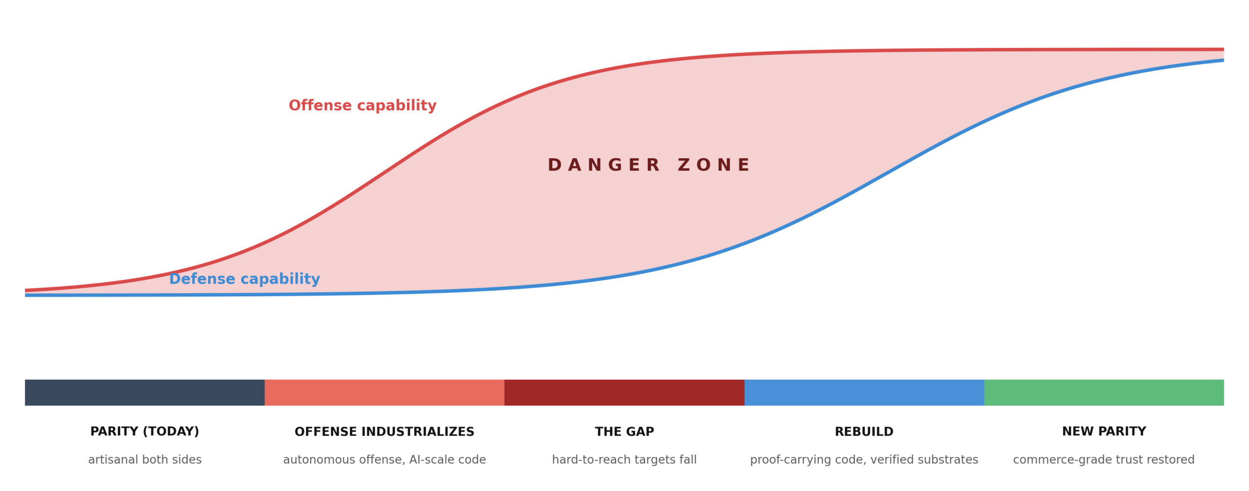
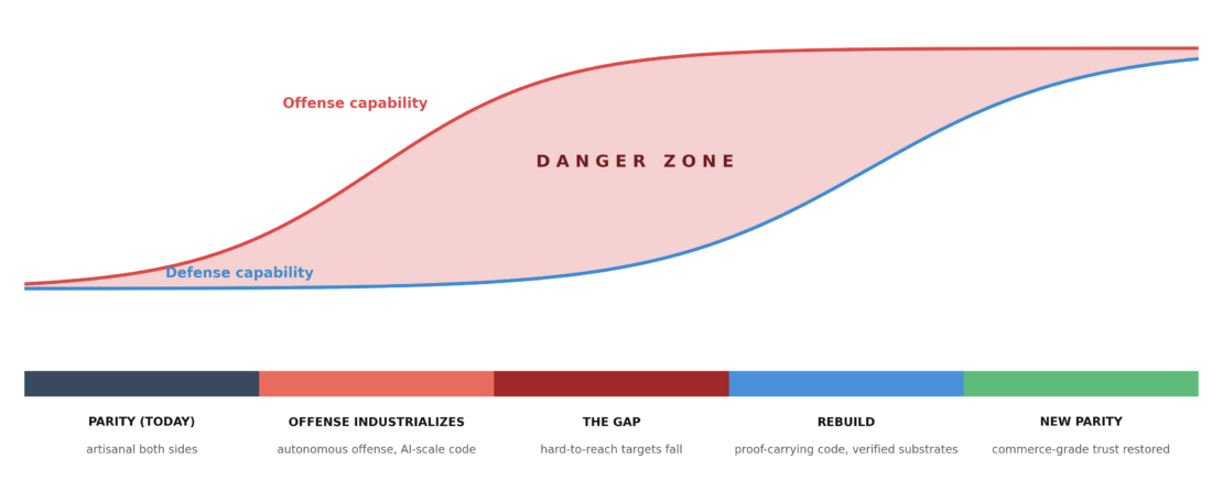
The result is a dangerous middle period — let’s call it “the period of excessive badness“. Attackers gain speed before defenders gain reliable automation. Vulnerability discovery accelerates before patching becomes autonomous. Attack campaigns become cheaper before institutions redesign authorities and workflows for machine-speed defense.

That is why the next few years are likely to be harder, not easier.

Offense spreads first. Autonomous exploitation collapses the marginal cost of finding and weaponizing a vulnerability, while AI-scale code production floods the stack with insecure software faster than humans ever shipped secure software. Defense has no symmetric productivity gain ready to deploy: formal verification, memory-safe substrates, and AI-native detection all exist as research or point tools, not as infrastructure. The result is a period of excessive badness — years in which the hard-to-reach parts of the digital world (OT, embedded systems, medical devices, legacy enterprise, firmware) pay the steepest price, because they cannot be patched on the cadence that industrialized offense now operates at. E-commerce-grade trust degrades, not uniformly, but in the places where the rebuild wave hasn’t reached.

Then comes the rebuild — paid for by the losses of the bad years, the way every prior security regime was paid for by its own catastrophe. Proof-carrying construction becomes the default for new code. Verification moves from a research artifact into the build pipeline. AI red-teaming runs continuously against every service. Hardware roots of trust, memory safety, and wide-scope AI defense get deployed as infrastructure, not features. What emerges is a new cyber parity that looks like today’s in shape — commerce works, banks work, the internet functions — but sits on a different substrate. The equilibrium holds not because attackers got worse, but because the floor got rebuilt. The policy question of this decade is not whether that end state arrives; it is how wide the gap is allowed to grow in the meantime, and which systems are sacrificed to the delay.

What This Means

The real cyber debate is usually framed in the wrong terms. People ask which vendor wins, which framework matters, or whether AI will replace analysts. Those are secondary. The first-order question is whether defenders can structurally attack the asymmetries that make offense easier — what tech is needed to correct this balance and how much damage accumulates before they do.

These are the questions I’m asking:

Can we compress the patch gap fast enough that working exploits do not enjoy a months-long free run?
Can we reduce the practical burden of defending millions of doors?
Can we make inevitable failures smaller, shorter, and cheaper?
Can we automate enough of defense that institutions are no longer asking humans to operate at a speed and scale humans were never built for?

The AISI evaluation of Mythos Preview is useful mostly because it puts a clock on those questions. Two years ago, frontier models could barely complete beginner tasks. Today, one of them can solve an end-to-end corporate attack simulation that costs a skilled human most of a workweek. The next generation will not be worse at it. Every month between here and a rebuilt substrate is a month the excessive-badness period gets a little wider — and a few more of the hard-to-reach systems (OT, embedded, medical devices, legacy enterprise, firmware) get quietly written off as unsalvageable.

The end state is plausible. Proof-carrying code, memory-safe foundations, continuous AI red-teaming, wide-scope AI defense running as infrastructure — these are research artifacts and point tools today, and they become substrate in the decade ahead. What is not yet decided is how wide the gap gets on the way there, and who pays for it. That is a policy question, not a technical one.

DEFCON may never look like the bolt convention I argued it should. But the realistic win isn’t boring — it’s bounded. A period of excessive badness that ends. A rebuild that shows up in time. A new parity we actually reach, on a different substrate than the one that got us here. That, more than any single breach or product cycle, is the real story of where cyber is headed.ns from abstractions into a timer. Two years ago, frontier models could barely complete beginner tasks. Today, one of them can solve an end-to-end corporate attack simulation that costs a skilled human most of a workweek. The next generation is unlikely to be worse at it. The phases above are not a leisurely roadmap. They are the order in which defenders have to show results before the offense-defense gap becomes structurally self-reinforcing.

If the answer to those questions is no, cyber will continue to feel like a field where defenders work harder each year only to hold less ground. If the answer is yes, the next decade could mark a genuine transition from artisanal defense to industrial defense.

That, more than any single breach or product cycle, is the real story of where cyber is headed.

Sources:

April 17, 2026 (updated July 9, 2026) By Tim Booher One Comment

Career & Productivity

Claude Code at Home

If you are lucky enough to have Claude code at work you get really spoiled. (I am.) You are the the bleeding edge of every update and can get an army of agents to tackle any problem. Unlike the real human world where we work a little, talk a little, get a cup of coffee and get back to work, the meter of token costs just keeps ticking.

And it’s expensive enough just to use power tools, but nothing works out of the box. You’re paying for the loop—the false starts, the “wait, let me open one more file,” the rewrite, the test, the cleanup, the second rewrite because the first rewrite wasn’t quite right. That loop is where real software gets built, and it’s also where credits vanish. It’s not that the models are overpriced in some abstract sense; it’s that the workflow is inherently iterative, and the billing model punishes iteration.

And the default model is to use the most expensive model for everything. While that’s convenient, it’s not what you should be doing at home when you have to choose between groceries or tokens.

Part of that is because these are days for being prodigal and testing a lot of things. You should be able to run things ten times in a row without feeling guilty. I want to chase a bug through a codebase, change my mind twice, and not have my brain doing mental math about whether I’m burning $8 or $80 today. I want to move fast, and I want the tool to be there the same way git is there—always available, always on, no drama.

But delegation is token-hungry by nature. The moment you let an agent do discovery—read files, skim configs, understand how tests run—you’ve entered the expensive zone. Not because the model is doing something complicated, but because the prompt becomes huge: policies, tool schemas, repo context, system instructions, plus your actual request. That’s before the model even starts thinking.

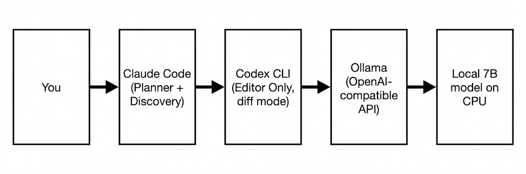
How do you actually pull this off? You let the strongest model be the boss and you assign everything else based on comparative advantage. For me that means Claude Code sits at the top as the supervisor and planner—it reads the repo, understands the architecture, and decides what needs to happen. OpenAI Codex lives one level down as the editor, taking tightly scoped instructions and producing clean diffs without wandering. And at the bottom is a locally running 7B Qwen 2.5 model through Ollama—CPU-bound, cheap, and always on—handling the boring, mechanical work. Judgment stays expensive and rare; execution becomes cheap and repeatable.

When I actually tried to do this, I found the bottleneck isn’t “can I run a model locally?” The bottleneck is “can I build a workflow that keeps my good tools while moving the expensive part out of the hot path?” Because you don’t want to give up Claude Code’s planning just to save money. You don’t want to give up Codex’s tight coding ergonomics either. You want to keep the good UI and the good behaviors, and just stop bleeding credits on every little edit.

That’s the problem statement in human terms: I want to use Claude and Codex like power tools, not like a casino meter. I want to delegate without anxiety. I want the loop back—fast iteration, lots of attempts, aggressive refactors—without that little voice saying “maybe don’t run it again.”

If you can solve that, you’re not just saving money. You’re restoring a way of working.

The good news is that the world is solving this problem. People have stopped thinking in terms of “pick one model” and started thinking in terms of “build a routing layer.” There’s been a genuine Cambrian explosion of models—open ones, semi-open ones, hosted ones—and developers are reacting the same way we always do when the ecosystem explodes: we put a gateway in front of it, normalize the interface, and swap engines behind the curtain. That’s why you see so much energy around OpenAI-compatible endpoints and proxies: you can point tools at one API shape and then decide later whether the request goes to Anthropic, OpenAI, Groq, a local Ollama box, or some hosted open model. LiteLLM is a clean example of this “gateway” pattern—one interface, lots of upstreams, plus routing/fallback ideas.

On the “hosted but cheaper” side, people are shopping for inference the way you shop for cloud compute: who can run decent models fast on specialized hardware at a lower price. Groq is the clearest “we are selling speed per dollar” play—very high token throughput and pricing that makes it attractive as a worker when you don’t need the absolute smartest model. OpenRouter is the marketplace version of the same instinct: one account, many models, and a routing/management layer so you can pick the right engine for the job (or let the router do it). They even publish guidance specifically about integrating Claude Code through their layer, which tells you how mainstream this “stick a router in front” approach has become.

Also popular are NVIDIA’s hosted endpoints, where you grab an NVIDIA API key and call models like Moonshot’s Kimi K2.5 through NVIDIA’s OpenAI-style chat/ completions interface. People mention it because it feels like cheating in the best way—GPU-backed inference, big context, modern agentic model, and the integration story is “just point your client at this base URL and use this model id.” NVIDIA’s own docs and blog posts are leaning into that exact pitch.

Meanwhile the other half of the world is going the opposite direction: “stop paying per token, I’ll run it myself.” Ollama on a workstation, LM Studio on a laptop, local quantized coding models, and a bunch of people stitching that into their editors so the ‘boring’ work has near-zero marginal cost. What’s interesting is that these two camps—cheap hosted inference and local inference—are converging on the same mental model: keep your premium model for judgment, and feed the grind to something cheaper, whether that’s a local box or a commodity inference provider. The tooling ecosystem is starting to assume you’ll do that, which is why everything is racing toward OpenAI-compatible APIs and “provider” abstractions.

What I ended up building is a split-brain workflow that feels obvious in hindsight: Claude stays in the driver’s seat as the planner and “reader,” and Codex becomes a local editor that only does the mechanical part—turning a very specific instruction into a clean diff. Under the hood, Codex isn’t talking to OpenAI at all; it’s pointed at an Ollama server running on the same machine, and Ollama is serving a small, cheap Qwen 2.5 7B model. The key design choice is that the local model never does discovery. It doesn’t roam your repo, it doesn’t decide what matters, it doesn’t try to be clever. Claude reads the codebase and decides exactly what should change; then it hands Codex a bounded edit task with the relevant file contents included, and Codex outputs a patch and stops. That’s the whole trick: you keep “judgment” expensive and rare, and you make “execution” cheap and repeatable.

To do this, install Ollama, then pull a model that’s small enough to be comfortable on CPU—Qwen 2.5 7B is a good starting point. The gotcha is that agentic tools like Codex have a surprisingly fat system prompt and tool schema, so a default 4k context model can choke in weird ways; the clean fix is to create a Codex-friendly variant with a larger context window. In Ollama that’s just a Modelfile and a new model name:

ollama pull qwen2.5:7b-instruct

cat > /tmp/Modelfile <<'EOF'
FROM qwen2.5:7b-instruct
PARAMETER num_ctx 12288
EOF

ollama create qwen2.5:7b-instruct-codex -f /tmp/Modelfile

Then you point Codex at Ollama using an OpenAI-compatible base URL, and you make sure Codex isn’t silently preferring cloud auth. Logging out of Codex cloud is the simplest way to prevent accidental spend, and then you set the config to use your local model by default:

codex logout 2>/dev/null || true

# ~/.codex/config.toml 
model = "qwen2.5:7b-instruct-codex"
model_provider = "ollama"

[model_providers.ollama]
name = "Ollama"
base_url = "http://localhost:11434/v1"
wire_api = "responses"

[projects."/home/tim"]
trust_level = "untrusted"

[projects."/home/tim/code"]
trust_level = "trusted"

At that point, a single command is enough to prove you’re local:

codex exec "Reply with exactly: WORKER_READY"

And the “how to actually use it” piece is mostly discipline: Claude does discovery and planning, and when it’s time to change code it produces one tight Codex command that includes the file content inline and says “output a unified diff only, then stop.” That sounds restrictive, but it’s what makes the whole thing fast and reliable on a 7B CPU worker—and it’s what turns the stack from a token furnace into something you can iterate with all day.

Now we get to the part that actually matters: was this worth it?

Because if this whole dance saves pennies but costs minutes, then it’s clever but not practical. So I ran the numbers across comparable tasks—real edits, real delegation loops—not toy prompts.

On cost alone, delegation works. It is dramatically cheaper than running everything through Opus, and marginally cheaper than just using Sonnet directly.

Average Cost Per Task

Approach	Avg Cost	vs Opus
Opus 4.6	$0.0779	baseline
Sonnet 4.5	$0.0139	82% cheaper
Delegated (Haiku + Codex)	$0.0135	83% cheaper

That’s not subtle. Opus is expensive. It’s phenomenal, but it’s expensive. Sonnet is already 82% cheaper than Opus for these tasks. Delegation edges Sonnet out by a hair—83% cheaper than Opus—but the difference between Sonnet and Delegated is basically noise.

The more interesting story is speed.

Average Time Per Task

Approach	Avg Time
Sonnet 4.5	10.2s
Opus 4.6	12.2s
Delegated	101.9s

Delegation is about 8.3× slower than just running Opus directly. And the bottleneck is exactly what you’d expect: Codex execution time on a local 7B CPU model. Once you leave the fast cloud inference path and move to a cheap worker, physics shows up. Thirty to one hundred twenty seconds per edit is normal.

So what does this mean in practice?

It means Sonnet 4.5 is a shockingly strong sweet spot. It’s almost as cheap as delegation—$0.0139 vs $0.0135 per task—and it’s an order of magnitude faster. If you’re optimizing purely for value per minute of your life, Sonnet direct execution is incredibly hard to beat.

Opus, meanwhile, is a premium product. At $0.0779 per task on average—5.6× more than Sonnet—it’s not what you use for mechanical edits. It’s what you use when you need the absolute best reasoning, when architecture matters, when ambiguity is high.

Now here’s the subtle part that changes the calculus: marginal cost.

When I tried to wire cloud Codex back into the stack, auth succeeded, the model resolved, and then I hit “quota exceeded.” That moment was clarifying. The architecture can’t depend on permission from a billing dashboard. If the middle layer disappears when credits run out, then it was never infrastructure — it was a subscription. So I reframed it: cloud Codex is an accelerator, not a dependency. The local worker is the default. Claude plans, the local model executes, and the system keeps running even if the cloud meter stops. If quota comes back, great — I get speed. If it doesn’t, nothing breaks. That shift — from rented capability to owned capability — is the difference between playing with AI and actually building with it.

So you end up with a very human tradeoff:

If you care about speed and you’re willing to pay $0.014 per task, Sonnet is phenomenal.

If you care about minimizing marginal cost and you can tolerate slower edits, delegation is almost free.

If you care about maximum reasoning quality, Opus is worth the premium.

The point of this architecture isn’t that delegation “wins” on every axis. It doesn’t. The point is that you now have control. You can route based on the task. You can pay for judgment and economize on repetition. You can choose whether you’re optimizing for time, money, or cognitive overhead.

And that’s the real unlock.

February 14, 2026 By Tim Booher 0 Comments

Personal Projects & Interests

Race Report for 2025 Dallas Marathon

Dallas Marathon (Dallas, TX) 2025-12-14

I pulled my race data into a database and did a technical teardown: pacing, mile splits, and heart-rate drift, plus a practical diagnosis of what happened in the last ~2 miles and what I should train so the last 10K feels better next time. Running is a constant-improvement sport and the data reveal exactly what happened during the race and what I could do better.

Summary

Ran 3:22:21 for 26.21 miles, with a +2:22 positive split (1:40:00 / 1:42:22). For me that’s still a good marathon: controlled pacing for most of the day, normal HR drift, and then a legs-first fade late instead of a full aerobic collapse. This race was fun, with the first 24 miles just a pure joy, wanting to run faster. The last two just hurt and that is what I dig into here.

The top-line story is a modest positive split: 1:40:00 / 1:42:22. Heart rate drifted upward in the second half (normal), and the pace only really falls off in the final miles — which matches how it felt.

Location	Dallas, TX
Date	2025-12-14
Start time	2025-12-14 09:00 EST
Distance	26.21 mi
Finish time (Workout.duration)	3:22:21
Moving time (Strava splits)	3:22:22
Elapsed time (Strava splits)	3:24:02
Elapsed time (stream timestamps)	3:20:57
Average pace (finish time)	7:43/mi
Avg / Max HR	151.7 / 172
Elevation gain	997 ft
Calories (Strava)	3210
Cadence (Strava)	84.9
Half split	1:40:00 / 1:42:22 (Δ 142s)
Pace steadiness (miles 2–26)	7:43/mi avg, 16.8s SD

Notes: Strava cadence is often reported as half of total steps/min for running (device-dependent). Mile splits + charts here use Strava’s per-mile moving-time splits; my earlier stream-derived splits were wrong because the imported timestamp/distance stream starts late and undercounts elapsed time.

Segment	Time	Avg Pace	Avg HR
First half	1:40:00	7:38/mi	146.5
Second half	1:42:22	7:49/mi	156.7

Graphs

I’m mostly using these as a sanity check: if the pace line stays flat while HR drifts up, that’s normal marathon fatigue. If the pace line starts spiking up late while HR stops rising, that usually points to my legs being the limiter.

Pace by Mile (min/mi)

This uses Strava’s per-mile moving-time splits (so it matches the app’s split table).

Average HR by Mile (bpm)

HR climbs in the second half even if pace is stable: normal marathon drift.

Mile Splits Table

My takeaway from the splits is “boringly consistent” for most of the day, with the meaningful slowdown concentrated late (miles 25–26). I’m including the full table because it’s the fastest way to see where the race actually changed.

Steadiness: miles 2–26 average pace 7:43/mi with split SD 16.8s. That’s a very controlled effort.

Mile	Split	Pace	Cum Time	Avg HR
1	7:35	7:35/mi	7:35	131.4
2	7:37	7:36/mi	15:12	143.3
3	7:39	7:39/mi	22:51	149.4
4	7:34	7:35/mi	30:25	144.0
5	7:38	7:37/mi	38:03	148.8
6	7:45	7:46/mi	45:48	149.1
7	7:44	7:44/mi	53:32	147.8
8	7:31	7:31/mi	1:01:03	148.5
9	7:35	7:35/mi	1:08:38	148.1
10	7:33	7:34/mi	1:16:11	143.2
11	7:46	7:45/mi	1:23:57	150.6
12	7:44	7:45/mi	1:31:41	148.1
13	7:29	7:29/mi	1:39:10	151.4
14	7:40	7:40/mi	1:46:50	151.9
15	7:42	7:42/mi	1:54:32	151.7
16	7:35	7:35/mi	2:02:07	153.2
17	7:37	7:36/mi	2:09:44	155.5
18	7:38	7:38/mi	2:17:22	156.3
19	8:00	8:00/mi	2:25:22	158.5
20	7:37	7:38/mi	2:32:59	163.7
21	7:29	7:28/mi	2:40:28	163.1
22	7:19	7:19/mi	2:47:47	161.4
23	7:38	7:38/mi	2:55:25	160.3
24	7:54	7:53/mi	3:03:19	157.5
25	8:17	8:17/mi	3:11:36	153.7
26	8:45	8:45/mi	3:20:21	152.7
27 (partial 0.212 mi)	2:01	9:32/mi	3:22:22	150.3

What Happened Late Race (the “legs got hard” part)

The race was controlled and just fun for a long time, but it’s a clear positive split overall, with the meaningful slowdown concentrated late. The final miles show a distinct pace drop while heart rate does not keep climbing. When my pace drops but HR doesn’t keep rising, I interpret that as a mechanical limiter: quads/calves/hip stability, stiffness, downhill damage, or just cumulative eccentric load — not a pure aerobic blow-up.

Concretely: I ran 1:40:00 / 1:42:22 (7:38/mi / 7:49/mi), and my average HR drifted from about 146.5 in the first half to about 156.7 in the second half — totally normal. The “it got really hard” part is still in the splits: mile 25 was 8:17 and mile 26 was 8:45, which are the slowest full miles.

Nutrition / Fueling Takeaways

I focused on nutrition, and the result strongly suggests it worked: a controlled marathon without a catastrophic fade is what good fueling often buys. I don’t have a precise gel-by-gel log in the data, but the next refinement is pretty standard and I can execute it intentionally next time.

My rule of thumb: start fueling earlier than I think I need to. The first hour protects the last hour. A reasonable target for a marathon effort is usually ~60–90g carbs/hour (gut tolerance dependent), and I want sodium/fluids consistent enough that I’m not inviting late cramping or that “stiff legs” feeling that shows up as pace decay.

Taper Autopsy

If I only look at the calendar, my taper looks reasonable. The DB says the last 14 days pre-race contained 35.2 miles across 14 run activities — but half of those are micro-activities (shorter than 0.75 miles or under 10 minutes). Filtering that noise out, I ran 31.5 “real” miles across 9 run-days in the final two weeks. That’s not “I stopped running.” It’s a normal reduction.

The more interesting story is intensity leakage. In the last 28 days pre-race, I logged three genuine stress runs at marathon-pace-ish or faster: D-22 was 18.14 miles at 7:45/mi (avg HR ~158), D-15 was 14.01 miles at 7:31/mi (avg HR ~154), and D-8 was 8.15 miles at 7:24/mi. Those aren’t insane workouts in isolation — but stacked inside the final three weeks, they make it harder to arrive with legs that feel springy at mile 25.

What I’d change next time: keep the routine the same, but back off the effort as race day gets close. Three weeks out is my last truly long run (18–20 miles, mostly easy, with a little marathon pace at the end only if I feel great). Two weeks out is a shorter long run (12–14) with just a small, controlled marathon‑pace segment, enough to stay sharp, not enough to beat up my legs. In the final 7–10 days, I want short reminders (strides and a few brief marathon‑pace reps), not an 8–10 mile run that quietly turns into a workout.

The point of taper isn’t to get fitter it’s to start the race rested enough to use the fitness I already built. That’s hard for me because I tend to do everything at full intensity, and I think that showed up here.

Actionable Next Steps (so the last 10K feels better)

My diagnosis is simple: my aerobic system was fine, but I didn’t have enough “fast running under fatigue” in the bank. The practical fix is to keep the long-run durability focus and add a repeatable dose of faster work (threshold and VO2-ish intervals) so marathon pace feels more like a gear I can hold late — not a gear I can hit early. That’s the missing piece when the last two miles went 8:17 and 8:45.

What my own training log says (DB-backed): in the 16 weeks before the race, I logged 399.3 miles of running (25.0 mpw average), but it was spiky (standard deviation 10.2 mpw; coefficient of variation 0.41), ranging from 8.6 miles in the lowest week to 46.9 miles in the biggest. I had 6 long runs ≥14 miles, only 3 ≥18, and just 1 ≥20 (a 23). That’s enough to run a respectable marathon, but it’s not a deep durability base for holding ~7:4x pace through mile 26, especially when some of the longest runs were already pretty demanding (e.g., 18.14 miles at 7:45/mi with avg HR ~158). My life is just too chaotic (travel every week, long hours and lots of different work from reserves to National Academies) and I needed to be more consistent to the plan versus lots of days of “let’s just get some miles in”.

What should have been different: fewer low weeks, more boring consistency. I want more weeks clustered in the 35–45 mpw range (instead of oscillating), plus one weekly threshold session and a long run that finishes at marathon pace every 2–3 weeks — while keeping the other long runs truly easy. In taper, I also want “pop without cost” (short marathon-pace touches + strides), not accidentally turning an 8–10 mile run into a sneaky hard effort. That combination is the cleanest way to make mile 25–26 feel like work instead of survival.

I’m not guessing on the “more speedwork” piece. A classic interval-training trial found that “High-aerobic intensity endurance interval training is significantly more effective than performing the same total work at either lactate threshold or at 70% HRmax, in improving VO2max” (Helgerud et al., 2007). A review on endurance determinants notes that “The speed at lactate threshold (LT) integrates all three of these variables and is the best physiological predictor of distance running performance” (Bassett & Howley, 2000). And on the durability/legs side, a strength-training review states: “Running economy is improved by performing combined endurance training with either heavy or explosive strength training” (Rønnestad & Mujika, 2014).

How I’m going to structure a typical week: two quality runs + one long run, with at least one truly easy day between stressors. If I’m stacking load (bigger mileage, more life stress, hot weather), I’ll run a two-week rotation and only do two hard sessions per week: one faster session + one long-run-specific session.

Workout 1: VO2-ish intervals (engine + form at speed): I’ll use the exact structure from that interval study because it’s simple and brutally effective: 4 × 4 minutes hard with 3 minutes easy jog recoveries (target ~90–95% HRmax by rep 2–3; pace usually around 3K–5K effort). Alternative when I want less strain: 6 × 3 minutes hard / 2 minutes easy, or 12 × 1 minute fast / 1 minute easy. Finish with 4–6 × 20s strides if my legs feel good.

Workout 2: Threshold / “comfortably hard” (raise the sustainable ceiling): this is the session I can hit almost every week without needing hero fitness. Options I like: 3 × 10 minutes at threshold with 2 minutes easy; 2 × 20 minutes at threshold with 3–5 minutes easy; or a steady 40-minute tempo if I’m in a good groove. Effort cue: strong, controlled, not gasping; I should finish thinking “I could do one more rep,” not “I’m cooked.”

Long run: specific durability (practice holding pace late): this is where I train the exact failure mode. The staple is a long run where marathon pace happens late, not early: 18–20 miles with the last 6–10 at marathon pace. If that’s too aggressive in a given week, I’ll do 3 × 4 miles at marathon pace inside a 20-miler (1 mile easy between), or a progression long run finishing the last 30–45 minutes at “steady/MP-ish.” The goal is to teach my legs to keep rhythm when they’d rather shuffle.

Strength (2×/week, short and non-negotiable): I’ll keep this boring and specific: split squats, step-downs, single-leg RDLs, calf raises (straight- and bent-knee), plus a little trunk/hip stability. Heavy-ish but clean reps, low volume, never to failure. The job is eccentric durability and stiffness, not soreness.

One constraint I’m going to respect: speedwork only helps if I absorb it. If my easy runs start drifting faster just to survive the week, I’ll cut volume before I cut quality, and I’ll keep at most two hard sessions in a 7-day window. Consistency beats a “perfect” spreadsheet week.

Overall, what a great day. I love marathon. I love the shared sacrifice, the distance, just long enough for a hard push. This time, I was a lot smarter with nutrition, getting in the miles and doing longer slow runs. Running and biking have been a consistent staple during an exceedingly chaotic time in my life and I’m super happy to have a nice race to end the season.

December 14, 2025 (updated December 15, 2025) By Tim Booher One Comment

Autonomy

AI Agents for Autonomy Engineers

This week I attended a DARPA workshop on the future and dimensions of agentic AI and also caught up with colleagues building flight-critical autonomy. Both communities use the word “autonomy,” but they mean different things. This post distinguishes physical autonomy (embodied systems operating in physics) from agentic AI (LLM-centered software systems operating in digital environments), and maps the design loops and tooling behind each. Full disclosure: I have real hands on experience building physically autonomous systems and am just learning how AI agents work so I’m more wordy in that section and hungry for feedback from actual AI engineers.

The DoW CTO recently consolidated critical technology areas, folding “autonomy” into “AI.” That may make sense at the budget level, but it blurs an important engineering distinction: autonomous physical systems are certified, safety-bounded, closed-loop control systems operating in the real world; agentic AI systems are closed-loop, tool-using software agents operating in digital workflows. For agentic digital systems, performance is the engineer’s goal. Physical systems are constrained by and designed for safety.

Both are feedback systems. The difference is what the loop closes over: physics (sensors → actuators) versus software (APIs → tool outputs). That single difference drives everything else: safety regimes, test strategies, and what failure looks like.

Physical autonomy (embodied AI)

Physical autonomy (often called “physical AI”) is intelligence embedded in robots, drones, vehicles, and other machines with a body. These systems don’t just predict; they act—and the consequences are kinetic. That’s why high-performing autonomy is not enough: the system must be safe under uncertainty.

Conceptually, autonomy is independence of action. Philosophically that’s old; engineering makes it concrete. In physical systems, “getting it wrong” can mean a crash, injury, or property damage—so the loop is designed to be bounded, testable, and auditable.

The physical loop (perceive → plan/control → act → learn)

Perceive. Sensors (camera, LiDAR, radar, GNSS/IMU, microphones) turn the world into signals. In practice, teams build low-latency perception pipelines around ROS 2, often with GPU acceleration (e.g., NVIDIA Isaac ROS / NITROS) and video analytics stacks (e.g., NVIDIA DeepStream).

Plan + control. Near safety-critical edges, autonomy still looks modular: perception → state estimation → planning → control. Classical tools remain dominant because they’re inspectable and constraint-aware (e.g., Nav2 for navigation; MPC toolchains like acados + CasADi when explicit constraints matter). Where LLM/VLA models help most today is at the higher level (interpreting goals, proposing constraints, generating motion primitives) while lower-level controllers enforce safety.

Act. Commands become motion through actuators and real-time control. Common building blocks include ros2_control for robot hardware interfaces and PX4 for UAV inner loops. When learned policies are deployed, they’re increasingly wrapped with safety enforcement (e.g., control barrier function “shielding” such as CBF/QP safety filters).

Learn. Physical autonomy improves through data: logs, simulation, and fleet feedback loops. Teams pair real logs with simulation (e.g., Isaac Lab / Isaac Sim) and rely on robust telemetry and replay tooling (e.g., Foxglove) to debug and improve perception and planning. The hard part is that real-world learning is constrained by cost, safety, and hardware availability.

Agentic AI (digital autonomy)

Agentic AI refers to LLM-centered systems that plan and execute multi-step tasks by calling tools, observing results, and re-planning—closing the loop over software workflows rather than physical dynamics.

External definitions help ground the term. The GAO describes AI agents as systems that can operate autonomously to accomplish complex tasks and adjust plans when actions aren’t clearly defined. NVIDIA similarly emphasizes iterative planning and reasoning to solve multi-step problems. In practice, the “agent” is the whole system: model + tools + memory + guardrails + evaluation.

The agent loop (perceive → reason → act → learn)

Perceive. Agents “sense” through connectors: files, web pages, databases, and APIs. Many production stacks use RAG (retrieval-augmented generation) so the agent can look up relevant documents before answering. That typically means embeddings + a vector database (e.g., pgvector/Postgres, Pinecone, Weaviate, Milvus, Qdrant) managed through libraries like LlamaIndex or LangChain.

Reason. This is the “autonomy” part in digital form: the system turns an ambiguous goal into a sequence of checkable steps, chooses a tool for each step, and updates the plan as results arrive. The practical trick is to move planning out of improvisational chat and into something you can debug and replay.

In production, that usually means a few concrete patterns: a planner/executor split (one component proposes a plan, another executes it—often as a planner that emits a structured plan (e.g., JSON steps with success criteria) and a constrained executor that runs one step at a time, enforces policy/permissions, and can reject a bad plan and trigger re-planning), an explicit state object (often JSON) that tracks what’s known, what’s pending, and what changed, and a workflow/graph that defines allowed transitions (including branches, retries, and “ask a human” escalations). Frameworks like LangGraph, Semantic Kernel, AutoGen, and Google ADK are popular largely because they make this structure first-class.

Mechanically, there’s no special parsing logic: the plan is parsed as normal JSON and validated against a schema (and often repaired by re-prompting if it fails). The executor is then a deterministic interpreter (a state machine / graph runner) that maps each step type to an allowed handler/tool, applies guards (required fields, permissions/approvals), and only then performs side effects.

Tooling-wise, the parts that matter most are: structured outputs (JSON schema / typed arguments), validators (e.g., schema checks and business rules), and failure policies (timeouts, backoff, idempotent retries, and fallbacks to a smaller/bigger model). That’s how “reasoning” becomes reproducible behavior instead of a clever one-off response.

Act. This is where an agent stops being “a good answer” and becomes “a system that does work.” Concretely, acting usually means calling an API (create a ticket, update a CRM record), querying a database, executing code, or triggering a workflow. The enabling tech is boring-but-critical: tool definitions with strict inputs/outputs (often JSON Schema or OpenAPI-derived), adapters/connectors to your systems, and a runtime that can execute calls, capture outputs, and feed them back into the loop. Standards like MCP are emerging to describe tools/connectors consistently across ecosystems.

The hard parts show up immediately: (1) tool selection (choosing the right function among many), (2) argument filling (mapping messy intent into typed fields without inventing values), and (3) side effects (a wrong call can email the wrong person, change the wrong record, or spend money). You also have to assume hostile inputs: prompt injection, tool-output “instructions,” and data exfiltration attempts. In practice, tool selection is usually a routing problem: you maintain a tool catalog (names, descriptions, schemas, permissions, cost/latency), retrieve a small candidate set (rules, embeddings, or a dedicated “router” model), then force the model to choose from that set (function calling / constrained output) and verify the choice (allowed tool? required approvals? inputs complete?) before executing. Production stacks handle this with layered defenses: validation and business-rule checks before execution, idempotency keys and backoff for retries, timeouts and circuit breakers for flaky dependencies, least-privilege auth (scoped tokens, service accounts), sandboxing/allow-lists for sensitive actions, explicit approvals for high-impact actions, and end-to-end observability (traces/logs so you can see what tool was called, with what arguments, and what happened).

Learn. Agent systems generate traces: prompts/messages, retrieved context, tool calls + arguments, tool outputs, decisions, and outcomes—stitched together with a trace ID. In production, this typically looks like structured logs + distributed tracing (often via OpenTelemetry), with redaction/PII controls and secure storage so you can share traces with humans without leaking secrets. The payoff is that traces become an eval dataset: you can sample failures, replay runs, and measure behavior (did it pick the right tool, ask for approval, respect policies, and terminate) using tooling such as OpenAI Evals, then iterate on prompts, routers, and (sometimes) fine-tuning.

Implementation patterns (one quick map)

If you’re building agents today, you’ll usually see one of two patterns: (1) graph/workflow orchestration (explicit steps and state; e.g., LangGraph) or (2) multi-agent role orchestration (specialized agents with handoffs; e.g., CrewAI, AutoGen, Semantic Kernel). Google’s ADK, OpenAI’s Agents SDK, and similar toolkits package these patterns with connectors, observability, and evaluation hooks.

Comparing autonomy: physics vs. software loops

Aspect	Physical autonomy	Agentic AI
What it operates on	Physics: sensors and actuators in messy environments	Software: APIs, documents, databases, and services
Loop constraints	Real-time latency, dynamics, and safety margins	Tool latency, reliability, and permission boundaries
Primary failure modes	Unsafe motion, collisions, degraded sensing, hardware faults	Wrong tool/arguments, prompt injection, bad data, silent side effects
How you test	Simulation + field testing + certification-style evidence	Evals + traces + sandboxing + staged rollout
Oversight	Often human-in-the-loop for safety-critical operations	On-the-loop monitoring with guardrails + approvals for risky actions

The loop is the same shape, but the domain changes everything: physics forces safety-bounded control; software forces permissions and security.
“Autonomy” isn’t a vibe: in both worlds it’s engineered feedback, measurable behavior, and an evidence trail.
Both converge on systems engineering: interfaces, observability, evaluation, and failure handling matter as much as model quality.

Where they merge (the payoff)

The most interesting systems blend the two: digital agents plan, coordinate, and monitor; embodied systems execute in the real world under strict safety constraints. You can already see this pattern in:

Robotics operations: agents triage logs, run diagnostics, and propose recovery actions while controllers enforce safety.
Warehouses and factories: agents schedule work and allocate resources; robots handle motion and manipulation.
Multi-robot coordination: agent-like planners coordinate tasks; low-level autonomy keeps platforms stable and safe.

Conclusion

Physical autonomy and agentic AI are two different kinds of independence: one closes the loop over physics, the other over software. Treating them as the same “AI” category hides the real engineering work: safety cases and control in the physical world; security, permissions, and eval-driven reliability in the digital world. The future is hybrid systems—but the way you build trust in them still depends on what the loop closes over.

December 13, 2025 (updated December 13, 2025) By Tim Booher 0 Comments

Engineering & Code

Memory‑Bound Inference: Why High‑Bandwidth Memory, Not FLOPs, Sets the Pace in AI – and What That Means for Blackwell vs. TPUs

It’s sunday night and NeurIPS is over. The Reagan National Defense Forum is over, and I’m sitting here in Fort Worth marinating in FOMO tracking the news from the weekend. Instead of live hallway conversations in San Diego or Simi Valley, my consolation prize is to deep dive into the hardware details that actually drive inference throughput. If Google is right that modern LLM inference is fundamentally High Bandwidth Memory (HBM)-bound, not FLOP-bound, then everything from how we value accelerators to how we think about “AI infrastructure” is subtly wrong—and that shift shows up very concretely in Blackwell’s bandwidth-first design and the walls TPUs are starting to hit.

At DARPA and Lockheed, I had to manage lots of various microelectronics programs and I’m really interested in how the economics of Google, Amazon, Tesla, Intel? and others are going to try to eat away at NVIDIA’s market share. My conclusion? This market share is not simple to grab and NVIDIA’s moat may actually be widening. This post reflects my personal views only and is not investment advice, and I am not a current professional expert in semiconductor or AI hardware equity analysis, so please do your own research before making any financial decisions.

Big programs and complex systems like the F-35 or the Boeing 737 live or die by the velocity of their supply chains. Good management is constantly obsessing over the theory of constraints as articulated by Goldratt. It’s helpful to look at a system and understand where the scarcity and abundance are and will be and then understand the drivers over time that will be the next gate you have to worry about.

Large language models (LLMs) and their transformer-based architecture have shifted the centre of gravity in AI hardware. A recent comment on X pointed out that if inference is truly HBM‑bound (as Google engineers themselves suggest), then the market has been modeling throughput incorrectly. This post dives into the technical reasons why floating point operations (FLOPs) alone don’t determine inference performance, explains why the industry’s “memory wall” has become the limiting factor, and examines how NVIDIA’s Blackwell architecture is designed around bandwidth and locality while even the newest TPU variants still struggle against the memory bottleneck.

The physics: compute scales faster than memory

Semiconductor scaling has delivered exponential growth in raw compute power, but memory capacity and bandwidth have lagged. An academic review of the “memory wall” notes that peak server FLOPS have been scaling roughly 3× every two years, whereas DRAM and interconnect bandwidth grow only ~1.6× and 1.4×, respectively. This divergence means that transferring data to the compute units is increasingly the bottleneck. The review argues that for many AI workloads the time to complete an operation is completely limited by DRAM bandwidth; no matter how fast arithmetic units are, they starve if data cannot be fed quickly.

Google’s infrastructure engineers echo this warning. Amin Vahdat wrote that advances in AI require redesigning the compute backbone because performance gains in computation have outpaced growth in memory bandwidth; simply adding compute units will cause them to idle while waiting for data. The first‑generation TPU design illustrates the point: Google admitted it was limited by memory bandwidth, so the second generation switched to High‑Bandwidth Memory (HBM) to increase bandwidth to 600 GB/s and double performance.

Why LLM inference is memory‑bandwidth bound

During LLM training, large batches reuse weights across many tokens, so arithmetic intensity is high and compute FLOPs dominate. Inference is different. Each token’s generation (decode) must fetch model weights and the per‑token key–value (KV) cache from HBM and write back updated KV states. A widely read technical guide shows that during generation, the arithmetic intensity of the attention block collapses: we perform a tiny matrix–vector multiply while streaming the entire KV cache. As a result we are basically always memory bandwidth‑bound during attention. The guide further notes that every sequence has its own KV cache, so larger batch sizes only increase memory traffic; we will almost always be memory‑bound unless architectures change. In concrete numbers, serving a 30B parameter model on a 4×4 TPU v5e slice (8.1 TB/s aggregate HBM bandwidth) yields a lower‑bound step time of 2.5 ms for a batch of four tokens, dominated by loading the weights and KV cache.

SemiAnalysis provides a similar picture. They explain that LLM inference repeatedly reads model weights and the KV cache from HBM and writes back the new key–value, and if bandwidth is insufficient, compute units sit idle. Consequently, most inference workloads are memory‑bandwidth bound. The report warns that increasing on‑chip FLOPs or even adding more HBM stacks does not eliminate the bottleneck because models expand to consume available memory (a “memory‑Parkinson” dynamic).

Roofline model of Nvidia A6000 GPU. The computation is in FP16

Even at the operator level, GPU microbenchmarks show that operations such as layer normalization, activations and attention remain HBM‑bound until sequence lengths of 4–16k tokens. AMD’s MI300X white paper likewise notes that many inference operations stay bandwidth‑limited until extremely large batches are used.

FLOPs versus memory bandwidth

In TPUs, each TensorCore contains a large matrix‑multiply unit (MXU), a vector unit and a very small on‑chip scratchpad (VMEM). Data must be copied from off‑chip HBM into VMEM before computation. The bandwidth between HBM and the TensorCore (typically 1–2 TB/s) limits how fast computation can be done in memory‑bound workloads. For matrix multiply operations (matmuls), the TPU architecture overlaps HBM loads with compute so that weight loads can be hidden, but for attention blocks this is not possible. When the load from HBM to VMEM is slower than the FLOPs in the MXU, the operation becomes bandwidth bound. Thus, adding more FLOPs does not improve throughput once the memory system is saturated.

These insights are why many accelerator researchers use arithmetic intensity (FLOPs per byte transferred) to model performance. For most LLM decode workloads the arithmetic intensity is low, so the throughput is proportional to the available memory bandwidth rather than the peak FLOPs. SemiAnalysis quantifies this: the MI300X, despite delivering over 5 PFLOPs of FP8 compute, is HBM‑bound for real‑world sequence lengths; the compute units simply cannot be saturated.

Evidence from Google: memory-optimized inference

Google’s own authors repeatedly acknowledge that inference is memory‑limited. The incredible DeepMind “How to Scale Your Model” (read it) series emphasizes that during generation, the attention block’s arithmetic intensity is constant and low; we’re doing a tiny amount of FLOPs while loading a massive KV cache. They advise that increasing batch size yields diminishing returns because each extra sequence adds its own KV cache. In follow‑up chapters describing Llama 3 inference on TPUs, the authors derive a 2.5 ms per‑step lower bound solely from HBM reads and note that for large KV caches we are well into the memory‑bound regime. When the KV cache fits into on‑chip VMEM, the decoder becomes compute‑bound, but in realistic models this rarely happens.

Google’s hardware roadmap also priotizes memory. The Ironwood TPU (v7) is marketed as “the first TPU for the age of inference.” In its technical brief, Google states that LLMs, Mixture‑of‑Experts and “thinking models” require massive parallel processing and efficient memory access. To support these workloads, Ironwood increases HBM capacity to 192 GB per chip (six times Trillium) and HBM bandwidth to 7.37 TB/s, “ensuring rapid data access [for] memory‑intensive workloads”. It also introduces a 1.2 TB/s bi‑directional inter‑chip interconnect to move data across thousands of chips. The emphasis is not on raw compute (although Ironwood delivers 4.6 TFLOP/s FP8 per chip), but on making sure data is always available to feed those compute units.

Even historical accounts underscore memory limitations. Wikipedia notes that Google stated the first‑generation TPU was limited by memory bandwidth, and that using 16 GB of HBM in the second generation increased bandwidth to 600 GB/s and greatly improved performance.

Blackwell: architecting around bandwidth and locality

While Google focuses on scaling out with many smaller chips, NVIDIA’s Blackwell GPUs (B200/B300) aim to maximise per‑chip throughput by radically redesigning the memory hierarchy. Key features include:

Massive on‑package HBM3e: The B200 integrates 192 GB of HBM3e delivering up to 8 TB/s of memory bandwidth. This is roughly four times the HBM bandwidth of H100 (2 TB/s ) and even exceeds the 7.37 TB/s of Google’s Ironwood .
Dual‑die design with 10 TB/s chip‑to‑chip link: Blackwell splits the GPU into two dies connected by a high‑speed interconnect delivering 10 TB/s of total bandwidth. This allows the memory system to be scaled without being limited by a single die’s package pins.
Huge unified L2 cache: Blackwell increases on‑chip cache to 192 MB (4× Hopper’s 48 MB) and uses a monolithic, unified L2 rather than multiple partitions. Microbenchmarking shows that this unified L2 delivers higher aggregate bandwidth at high concurrency, making it ideal for bandwidth‑bound applications like deep‑learning inference.
Tensor Memory (TMEM) and locality‑aware hierarchy: Each Tensor Core has a local “TMEM” with tens of terabytes per second of bandwidth. Data flows from TMEM (~100 TB/s) to L1/shared memory (~40 TB/s) to L2 (~20 TB/s) and only then to HBM (~8 TB/s), ensuring most accesses hit faster caches. This hierarchical design keeps compute busy by maximizing locality.

SemiAnalysis observes that HBM capacity and bandwidth are exploding in Blackwell and other next‑gen GPUs – from ~80 GB in Hopper to up to 1 TB per chip by 2027 – and that memory now dominates bill‑of‑materials cost. They warn that as HBM grows, models will consume it, so memory remains the limiting factor. Blackwell’s architecture directly addresses this by centring the design on bandwidth and cache, not just compute.

TPUs and the memory wall

TPUs use systolic arrays to achieve enormous matrix‑multiply throughput, but their memory hierarchy is shallow. For inference chips like TPU v5e, the HBM bandwidth is about 8.1 TB/s aggregate across a 16‑chip slice; each chip has roughly 1–2 TB/s of HBM bandwidth. Without enough bandwidth, the MXUs idle. This is why the DeepMind guides emphasize prefetching weights into VMEM and using techniques like FlashAttention; but they still conclude that attention during generation is always memory‑bandwidth bound .

Ironwood improves HBM bandwidth to 7.37 TB/s per chip and scales to pods of 9,216 chips. However, even this may not be enough for frontier LLMs: a 70 B parameter model with 100 kB per‑token KV cache and typical batch sizes can consume tens of gigabytes of bandwidth per token. A case study on serving Llama 3 shows that decode throughput on TPU v5e is limited to ~235 tokens/s per chip due to the time to stream weights and KV cache from HBM. Increasing compute or using lower precision (INT8/FP8) does not help once memory saturates. Unlike GPUs, TPUs also lack large unified caches; each core has only ~128 MiB of VMEM , so large weights cannot be prefetched.

Comparing accelerators on memory capacity and bandwidth

Accelerator	HBM capacity (per chip)	HBM bandwidth (per chip)	Notable memory features
NVIDIA H100 (Hopper)	80GB HBM3	3 TB/s bandwidth for the SXM version	60MB L2 cache
NVIDIA Blackwell B200	192 GB HBM3e	8 TB/s	50MB L2 cache
B300	288GB HBM3e	8 TB/s	??
Google TPU v7 (Ironwood)	192 GB HBM3e	7.37 TB/s	1.2 TB/s bi‑directional inter‑chip interconnect; architecture focuses on minimizing data movement
AMD MI300X	192 GB HBM3	5.3 TB/s	8‑GPU board with 128 GB/s Infinity Fabric between GPUs

The table highlights that Blackwell offers the highest per‑chip bandwidth and combines it with a large on‑chip cache. Ironwood and MI300X have similar memory capacity but less bandwidth; H100 lags both in capacity and bandwidth. These differences matter more than raw compute because inference throughput scales with the numerator (bandwidth) rather than the denominator (FLOPs). For example, a Blackwell B200 can stream more than 8 × 10¹² bytes per second, enough to feed its Tensor Cores when decoding many tokens in parallel, whereas an H100’s 2 TB/s often becomes the bottleneck for large KV caches.

Market implications: HBM vendors and Nvidia’s widening moat

If inference performance is constrained by memory bandwidth, the supply and cost of HBM become central. SemiAnalysis argues that the exploding HBM capacity and bandwidth are making memory the dominant cost driver in AI accelerators. As new architectures triple or quadruple the HBM per chip, the number of stacked DRAM dies and the complexity of through‑silicon vias increase; only a handful of manufacturers (Samsung, SK Hynix, Micron) can produce high‑stack HBM at scale. Micron’s 2026 investment in a $9.6 billion HBM fab underscores how strategic this market has become. Chips with superior bandwidth will fetch premium prices, but they depend on a constrained supply chain.

For Nvidia, memory‑bound inference amplifies its competitive advantages:

Architectural moat: Blackwell’s memory‑centric design (large L2, TMEM, dual‑die interconnect) means that even with equivalent compute, competing chips may not feed their cores fast enough. Microbenchmarks show that the unified L2 on GB203 delivers higher aggregate bandwidth at high concurrency, making it particularly well‑suited for bandwidth‑bound deep‑learning inference .
Interconnect and software moat: NVLink/NVSwitch networks provide up to 1.8 TB/s per link (on Blackwell NVLink 5) and allow memory pooling across GPUs. The high‑bandwidth NVLink network, combined with optimized software (CUDA, cuDNN, TensorRT‑LLM), overlaps HBM, L2 and NVLink transfers to maximize throughput.
HBM scale: Nvidia collaborates closely with HBM vendors and invests in co‑packaged memory. Blackwell’s design requires extremely high stacking (12–Hi HBM3e) and advanced packaging. As memory becomes the bottleneck, chips that integrate more HBM stacks with high‑yield packaging will command a premium.
Ecosystem: Blackwell GPUs can be deployed today; Google’s Ironwood and AMD’s MI300X are currently available only through cloud or limited channels. Many AI researchers and enterprises already invest in Nvidia’s software stack; switching to alternative accelerators requires rewriting code or retraining models.

From this perspective, HBM vendors win because memory, not compute, dictates throughput. The limited pool of HBM suppliers can extract higher margins, and chipmakers without strong relationships will struggle to scale. Nvidia’s moat widens because Blackwell’s memory‑centric architecture and NVLink network directly address the inference bottleneck. Google’s TPUs push bandwidth higher but still face the memory wall; the DeepMind guides explicitly caution that attention blocks are always memory‑bound and that throughput scales with HBM bandwidth. Unless Google can radically redesign the memory hierarchy or deploy far larger pods, their per‑chip throughput remains capped by HBM supply.

Conclusion

Inference in large language models is not about raw FLOPs. It is about how fast you can stream parameters and key‑value caches from memory into the compute units. Evidence from academic analyses, industry insiders and Google’s own documentation shows that most LLM inference workloads are memory‑bandwidth bound, not compute‑bound. The memory wall arises because DRAM and interconnect bandwidth scale much more slowly than compute, so even adding more compute units or using lower precisions does not increase throughput .

Blackwell’s architecture reflects this reality: huge HBM3e stacks, unified L2 cache, high‑speed chiplets and a locality‑aware hierarchy combine to maximize effective bandwidth. Google’s Ironwood TPU improves memory capacity and bandwidth but still emphasizes high‑bandwidth interconnects to hide memory latency. AMD’s MI300X offers large HBM capacity but less bandwidth. When comparing accelerators, the correct metric is bytes/s per chip rather than teraflops; as the table shows, Blackwell leads on bandwidth.

Investors and technologists should therefore model inference throughput based on memory capacity and bandwidth, not on peak FLOPs. In this memory‑bound world, HBM suppliers become strategic winners, and NVIDIA’s investment in memory‑centric architectures deepens its competitive moat. The age of abundant compute is here; the age of abundant memory is not – and that is where the next battle in AI acceleration will be fought.

December 7, 2025 (updated December 15, 2025) By Tim Booher 0 Comments

Autonomy

AI and Aerodynamics at Insect Scale: MIT’s Bumblebee‑Sized Robot

MIT soft robotics lab did an amazing job right at the intersection of physical systems, cyber and software. Small robots and insect-related autonomy have fascinated me for awhile. The autonomy of an insect brain is simple enough to just start to touch the boundaries of AI. The aero and mechanics of insects is still mind-bendingly ahead of our best planes (power, maneuver, agility, range).

MIT’s latest insect-scale robot fuses new soft “muscle” actuators, a redesigned four-wing airframe, and an AI-trained controller to achieve truly bug-like flight. Multi-layer dielectric elastomer actuators provide high power at much lower voltage, while long, hair-thin wing hinges and improved transmissions cut mechanical stress so the robot can hover for about 1,000 seconds and execute flips and sharp turns faster than previous microrobots. On top of that hardware, the team uses model-predictive control as an expert “teacher” and distills it into a lightweight neural policy, enabling bumblebee-class speed and agility in a package that weighs less than a paperclip and opens a realistic path to autonomous swarms for pollination and search-and-rescue.

Tiny flying robots have long promised to help with tasks that are too dangerous or delicate for larger drones. Building such machines is extraordinarily difficult: the physics of flapping‑wing flight at insect scale and the constraints of small motors and batteries limit endurance and manoeuvrability. Over the past four years, engineers at the Massachusetts Institute of Technology (MIT) have made three major breakthroughs that together push insect‑scale flight from lab curiosity toward practical autonomy.

I built an animation using three.js to show just how cool this flight path can be.

The insect’s flight path is modeled using a discrete-time Langevin equation, which simulates Brownian motion with aerodynamic damping. At each time step $ t $, the velocity vector $ \mathbf{v} $ is updated by applying a stochastic acceleration $ \mathbf{a}_{\text{rand}} $ and a damping factor $ \gamma $ (representing air resistance):
$$ v_{t+1} = \gamma \, v_t + \mathbf{a}_{\text{rand}} $$
where $ \gamma = 0.95 $ and the components of $ \mathbf{a}_{\text{rand}} $ are drawn from a uniform distribution $ \mathcal{U}(-0.05, 0.05) $. The position $ \mathbf{p} $ is then integrated numerically:
$$ \mathbf{p}_{t+1} = \mathbf{p}_t + \mathbf{v}_{t+1} $$
This results in a “random walk” trajectory that is smoothed by the inertial momentum of the simulated robot, mimicking the erratic yet continuous flight dynamics of a small insect.

Use mouse to rotate/zoom.

Flying robots smaller than a few grams operate in a very different aerodynamic regime from traditional drones. Their wings experience low Reynolds numbers where lift comes from unsteady vortex shedding rather than smooth airflow; getting useful thrust requires wings to flap hundreds of times per second with large stroke angles. At such high frequencies, actuators often buckle and joints fatigue. The robots have extremely tight power and mass budgets, making it hard to carry batteries or onboard processors. Early insect‑like microrobots could just barely hover for a few seconds and needed bulky external power supplies.

A microrobot flips 10 times in 11 seconds.
Credit: Courtesy of the Soft and Micro Robotics Laboratory

MIT’s Soft and Micro Robotics Laboratory, led by Kevin Chen, set out to tackle these problems with a combination of novel soft actuators, mechanically resilient airframes and advanced control algorithms. The resulting platform evolved in three stages: improved artificial muscles (2021), a four‑wing cross‑shaped airframe with durable hinges and transmissions (January 2025) and a learning‑based controller that matches insect agility (December 2025).

The first breakthrough addressed the “muscle” problem. Conventional rigid actuators were too heavy and inefficient for gram‑scale robots. Chen’s group developed multilayer dielectric elastomer actuators—soft “muscles” made from ultrathin elastomer films sandwiched between carbon‑nanotube electrodes and rolled into cylinders. In 2021 they unveiled a fabrication method that eliminates microscopic air bubbles in the elastomer by vacuuming each layer after spin‑coating and baking it immediately. This allowed them to stack 20 alternating layers, each about 10 µm thick , without defects.

Key results from this work included:

Lower voltage and more payload: The new actuators operate at 75% lower voltage and carry 80% more payload than earlier soft actuators. By increasing surface area with more layers, they require less than 500V to actuate yet can lift nearly three times their own weight.
Higher power density and durability: Removing defects increases power output by more than 300% and extends lifespan. The 20‑layer actuators survived more than 2 million cycles while still flying smoothly.
Record hovering: Robots powered by these actuators achieved a 20‑second hovering flight, the longest yet recorded for a sub‑gram robot. With a lift‑to‑weight ratio of about 3.7:1, they could carry additional electronics.

The low‑voltage soft muscles solved a critical bottleneck: the robots could now carry lightweight power electronics and eventually microprocessors instead of being tethered to an external power supply. This breakthrough laid the hardware foundation for future autonomy.

Aerodynamic and structural redesign: four wings, durable hinges and long endurance

The second breakthrough came in early 2025 with a redesign of the robot’s wings and transmission. Previous generations assembled four two‑wing modules into a rectangle, creating eight wings whose wakes interfered with each other and limiting control authority. The new design arranges four single‑wing units in a cross. Each wing flaps outward, reducing aerodynamic interference and freeing up central volume for batteries and sensors.

To exploit the power of the improved actuators, Chen’s team built more complex transmissions that connect each actuator to its wing. These transmissions prevent the artificial muscles from buckling at high flapping frequencies, reducing mechanical strain and allowing higher torque. They also developed a 2 cm‑long wing hinge with a diameter of just 200 µm, fabricated via a multistep laser‑cutting process. The long hinge reduces torsional stress during flapping and increases durability; even slight misalignment during fabrication could affect the wing’s motion.

Performance improvements from this structural redesign were dramatic:

Extended flight time: The robot can hover for more than 1,000 seconds (~17 minutes) without degradation of precision —100 times longer than earlier insect‑scale robots.
Increased speed and agility: It reaches an average speed of 35 cm/s and performs body rolls and double flips. It can precisely follow complex paths, including spelling “MIT” in mid‑air.
Greater control torque: The new transmissions generate about three times more torque than prior designs , enabling sophisticated and accurate path‑following flights.

These mechanical innovations show how aerodynamic design, materials engineering and manufacturing precision are intertwined. By reducing strain on the wings and actuators, the platform gains not only endurance but also the stability needed for advanced control.

Autonomy, AI and Systems Engineering

The final breakthrough is in control theory as it intersects autonomy. Insect‑scale flight demands rapid decision‑making: the wings beat hundreds of times per second, and disturbances like gusts can quickly destabilize the robot. Traditional hand‑tuned controllers cannot handle aggressive maneuvers or unexpected perturbations. MIT’s team collaborated with Jonathan How’s Aerospace Controls Laboratory to develop a two‑step AI‑based control scheme.

Step 1: Model‑predictive control (MPC). The researchers built a high‑fidelity dynamic model of the robot’s mechanics and aerodynamics. An MPC uses this model to plan an optimal sequence of control inputs that follow a desired trajectory while respecting force and torque limits. The planner can design difficult maneuvers such as repeated flips and aggressive turns but is too computationally intensive to run on the robot in real time.

Step 2: Imitation‑learned policy. To bridge the gap between high‑end planning and onboard execution, the team generated training data by having the MPC perform many trajectories and perturbations. They then trained a deep neural network policy via imitation learning to map the robot’s state directly to control commands. This policy effectively compresses the MPC’s intelligence into a lightweight model that can run fast enough for real‑time control.

The results show how AI enables insect‑like agility:

Speed and acceleration: The learning‑based controller allows the robot to fly 447% faster and achieve a 255% increase in acceleration compared with their previous best hand‑tuned controller.
Complex maneuvers: The robot executed 10 somersaults in 11 seconds, staying within about 4–5 cm of the planned trajectory and maintaining performance despite wind gusts of more than 1 m/s
Bio‑inspired saccades: The policy enabled saccadic flight behavior, where the robot rapidly pitches forward to accelerate and then back to decelerate, mimicking insect eye stabilization strategies.

An external motion‑capture system currently provides state estimation, and the controller runs offboard. However, because the neural policy is much less computationally demanding than full MPC, the authors argue that similar policies may be feasible on tiny onboard processors. The AI control thus paves the way for autonomous flight without external assistance.

A key message of MIT’s microrobot program is that agility at insect scale does not come from a single innovation. The soft actuators enable large strokes at lower voltage; the cross‑shaped airframe and long hinges reduce mechanical strain and aerodynamic interference; and the AI‑driven controller exploits the robot’s physical capabilities while respecting constraints. Chen’s group emphasizes that hardware advances pushed them to develop better controllers, and improved controllers made it worthwhile to refine the hardware.

This co‑design philosophy—optimizing materials, mechanisms and algorithms together—will be essential as researchers push toward untethered, autonomous swarms. The team plans to integrate miniature batteries and sensors into the central cavity freed by the four‑wing design, allowing the robots to navigate without a motion‑capture system. Future work includes landing and take‑off from flowers for mechanical pollination and coordinated flight to avoid collisions and operate in groups. There are also open questions about enabling onboard perception—using tiny cameras or event sensors to close the loop—and about energy management to extend endurance beyond 10,000s.

MIT’s bumblebee‑sized flapping robot illustrates how progress in materials science, precision fabrication, aerodynamics and AI can converge to solve a hard problem. The low‑voltage, power‑dense actuators prove that soft materials can outperform rigid designs, the four‑wing airframe with durable hinges unlocks long endurance and high torque, and the hybrid MPC/learning controller shows that sophisticated planning can be compressed into hardware‑friendly neural policies. Together, these advances give the microrobot insect‑like speed, agility and endurance.

While still reliant on external power and motion capture, the robot’s modular design and AI controller suggest a roadmap to fully autonomous operation. As the team integrates onboard sensors and batteries, insect‑scale robots could move from labs to fields and disaster zones, pollinating crops or searching collapsed buildings. In that future, the intersection of autonomy and aerodynamics will be defined not by a single breakthrough but by a careful co‑design of muscles, wings and brains.

December 6, 2025 (updated December 7, 2025) By Tim Booher One Comment

Autonomy

AI Hackers

AI Systems Are Now Hunting Software Vulnerabilities—And Winning.

Three months ago, Google Security SVP Heather Adkins and cryptographer Bruce Schneier warned that artificial intelligence would unleash an “AI vulnerability cataclysm.” They said autonomous code-analysis systems would find and weaponize flaws so quickly that human defenders would be overwhelmed. The claim seemed hyperbolic. Yet October and November of 2025 have proven them prescient: AI systems are now dominating bug bounty leaderboards, generating zero-day exploits in minutes, and even rewriting malware in real time to evade detection.

On an October morning, a commercial security agent called XBOW—a fully autonomous penetration tester—shot to the top of HackerOne’s U.S. leaderboard, outcompeting thousands of human hackers. Over the previous 90 days it had filed roughly 1,060 vulnerability reports, including remote-code-execution, SQL injection and server-side request forgery bugs. More than 50 were deemed critical. “If you’re competing for bug bounties, you’re not just competing against other humans anymore,” one veteran researcher told me. “You’re competing against machines that work 24/7, don’t get tired and are getting better every week.”

XBOW is just a harbinger. Between August and November 2025, at least nine developments upended how software is secured. OpenAI, Google DeepMind and DARPA all released sophisticated agents that can scan vast codebases, find vulnerabilities and propose or even automatically apply patches. State-backed hackers have begun using large-language models to design malware that modifies itself in mid-execution, while researchers at SpecterOps published a blueprint for an AI-mediated “gated loader” that decides whether a payload should run based on a covert risk assessment. And an AI-enabled exploit generator published in August showed that published CVEs can be weaponized in 10 to 15 minutes—collapsing the time defenders once had to patch systems.

The pattern is clear: AI systems aren’t just assisting security professionals; they’re replacing them in many tasks, creating new capabilities that didn’t exist before and forcing a fundamental rethinking of how software security works. As bug-bounty programs embrace automation and threat actors deploy AI at every stage of the kill chain, the offense-defense balance is being recalibrated at machine speed.

A New Offensive Arsenal

The offensive side of cybersecurity has seen the most dramatic AI advances, but it’s important to understand the distinction between what’s happening: foundational model companies like OpenAI and Anthropic are building the brains, while agent platforms like XBOW are building the bodies. This distinction matters when evaluating the different approaches emerging in AI-powered security.

OpenAI’s Aardvark, released on Oct. 30, is described by the company as a “security researcher” in software form. Rather than using static analysis or fuzzers, Aardvark uses large-language-model reasoning to build an internal representation of each codebase it analyzes. It continuously monitors commits, traces call graphs and identifies risky patterns. When it finds a potential vulnerability, Aardvark creates a test harness, executes the code in a sandbox and uses Codex to propose a patch. In internal benchmarks across open-source repositories, Aardvark reportedly detected 92 percent of known and synthetic vulnerabilities and discovered 10 new CVE-class flaws. It has already been offered pro bono to select open-source projects. But beneath the impressive numbers, Aardvark functions more like AI-enhanced static application security testing (SAST) than a true autonomous researcher—powerful, but incremental.

Google DeepMind’s CodeMender, unveiled on Oct. 6, takes the concept further by combining discovery and automated repair. It applies advanced program analysis, fuzzing and formal methods to find bugs and uses multi-agent LLMs to generate and validate patches. Over the past six months, CodeMender upstreamed 72 security fixes to open-source projects, some as large as 4.5 million lines of code. In one notable case, it inserted -fbounds-safety annotations into the WebP image library, proactively eliminating a buffer overflow that had been exploited in a zero-click iOS attack. All patches are still reviewed by human experts, but the cadence is accelerating.

Anthropic, meanwhile, is taking a fundamentally different path—one that involves building specialized training environments for red teaming. The company has devoted an entire team to training a foundational red team model. This approach represents a bet that the future of security AI lies not in bolting agents onto existing models, but in training models from the ground up to think like attackers.

The DARPA AI Cyber Challenge (AIxCC), concluded in October, showcased how far autonomous systems have come. Competing teams’ tools scanned 54 million lines of code, discovered 77 percent of synthetic vulnerabilities and generated working patches for 61 percent—with an average time to patch of 45 minutes. During the final four-hour round, participants found 54 new vulnerabilities and patched 43, plus 18 real bugs with 11 patches. DARPA announced that the winning systems will be open-sourced, democratizing these capabilities.

A flurry of attack-centric innovations soon followed. In August, researchers demonstrated an AI pipeline that can weaponize newly disclosed CVEs in under 15 minutes using automated patch diffing and exploit generation; the system costs about $1 per exploit and can scale to hundreds of vulnerabilities per day. A September opinion piece by Gadi Evron, Heather Adkins and Bruce Schneier noted that over the summer, autonomous AI hacking graduated from proof of concept to operational capability. XBOW vaulted to the top of HackerOne, DARPA’s challenge teams found dozens of new bugs, and Ukraine’s CERT uncovered malware using LLMs for reconnaissance and data theft, while another threat actor was caught using Anthropic’s Claude to automate cyberattacks. “AI agents now rival elite hackers,” the authors wrote, warning that the tools drastically reduce the cost and skill needed to exploit systems and could tip the balance towards the attackers.

Yet XBOW’s success reveals an important nuance about agent-based security tools. Unlike OpenAI’s Aardvark or Anthropic’s foundational approach, XBOW is an agent platform that uses these foundational models as backends. The vulnerabilities it finds tend to be surface-level—relatively easy targets like SQL injection, XSS and SSRF—not the deep architectural flaws that require sophisticated reasoning. XBOW’s real innovation wasn’t its vulnerability discovery capability; it was using LLMs to automatically write professional vulnerability reports and leveraging HackerOne’s leaderboard as a go-to-market strategy. By showing up on public rankings, XBOW demonstrated that AI could compete with human hackers at scale, even if the underlying vulnerabilities weren’t particularly complex.

Defense Gets More Automated—But Threats Evolve Faster

Even as defenders deploy AI, adversaries are innovating. The Google Threat Intelligence Group (GTIG) AI Threat Tracker, published on Nov. 5, is the most comprehensive look to date at AI in the wild. For the first time, GTIG identified “just-in-time AI” malware that calls large-language models at runtime to dynamically rewrite and obfuscate itself. One family, PROMPTFLUX, is a VBScript dropper that interacts with Gemini to generate new code segments on demand, making each infection unique. PROMPTSTEAL is a Python data miner that uses Qwen2.5-Coder to build Windows commands for data theft, while PROMPTLOCK demonstrates how ransomware can employ an LLM to craft cross-platform Lua scripts. Another tool, QUIETVAULT, uses an AI prompt to search JavaScript for authentication tokens and secrets. All of these examples show that attackers are moving beyond the 2024 paradigm of AI as a planning aide; in 2025, malware is beginning to self-modify mid-execution.

GTIG’s report also highlights the misuse of AI by state-sponsored actors. Chinese hackers posed as capture-the-flag participants to bypass guardrails and obtain exploitation guidance; Iranian group MUDDYCOAST masqueraded as university students to build custom malware and command-and-control servers, inadvertently exposing their infrastructure. These actors used Gemini to generate reconnaissance scripts, ransomware routines and exfiltration code, demonstrating that widely available models are enabling less-sophisticated hackers to perform advanced operations.

Meanwhile, SpecterOps researcher John Wotton introduced the concept of an AI-gated loader, a covert program that collects host telemetry—process lists, network activity, user presence—and sends it to an LLM, which decides whether the environment is a honeypot or a real victim. Only if the model approves does the loader decrypt and execute its payload; otherwise it quietly exits. The design, dubbed HALO, uses a fail-closed mechanism to avoid exposing a payload in a monitored environment. As LLM API costs fall, such evasive techniques become more practical.

Consolidation and Friction

These technological leaps are reshaping the business of cybersecurity. On Nov. 4, Bugcrowd announced that it will acquire Mayhem Security from my good friend David Brumley. His team was previously known as ForAllSecure and won the 2016 DARPA Cyber Grand Challenge. Mayhem’s technology automatically discovers and exploits bugs and uses reinforcement learning to prioritize high-impact vulnerabilities; it also builds dynamic software bills of materials and “chaos maps” of live systems. Bugcrowd plans to integrate Mayhem’s AI automation with its human hacker community, offering continuous penetration testing and merging AI with crowd-sourced expertise. “We’ve built a system that thinks like an attacker,” Mayhem founder David Brumley said, adding that combining with Bugcrowd brings AI to a global hacker network. The acquisition signals that bug bounty platforms will not remain purely human endeavours; automation is becoming a product feature.

The Mayhem acquisition also underscores the diverging strategies in the AI security space. While agent platforms like XBOW focus on automation at scale, foundational model teams are making massive capital investments in training infrastructure. Anthropic’s multi-billion-dollar commitment to building specialized red teaming environments dwarfs the iterative approach seen elsewhere. This created substantial competitive pressure: when word spread that Anthropic was spending at this scale, it generated significant fear of missing out among both startups and established players, accelerating consolidation moves like the Bugcrowd-Mayhem deal.

Yet adoption is uneven. Some folks I spoke with are testing Aardvark and CodeMender for internal red-teaming and patch generation but won’t deploy them in production without extensive governance. They worry about false positives, destabilizing critical systems and questions of liability if an AI-generated patch breaks something. The friction isn’t technological; it’s organizational—legal, compliance and risk management must all sign off.

The contrast between OpenAI’s and Anthropic’s approaches is striking. OpenAI’s Aardvark, while impressive in benchmarks, functions primarily as enhanced SAST—using AI to improve traditional static analysis rather than fundamentally rethinking how security research is done. Anthropic, by contrast, is betting that true autonomous security research requires training foundational models specifically for offensive security, complete with vast training environments that simulate real-world attack scenarios. This isn’t just a difference in tactics; it’s a philosophical divide about whether security AI should augment existing tools or replace them entirely.

Attackers, by contrast, face no such constraints. They can run self-modifying malware and LLM-powered exploit generators without worrying about compliance. GTIG’s report notes that the underground marketplace for illicit AI tooling is maturing, and the existence of PROMPTFLUX and PROMPTSTEAL suggests some criminal groups are already paying to call LLM APIs in operational malware. This asymmetry raises an unsettling question: Will AI adoption accelerate faster on the offensive side?

What Comes Next

Experts outline three scenarios. The Slow Burn assumes high friction on both sides leads to gradual, manageable adoption, giving regulators and organizations time to adapt. An Asymmetric Surge envisions attackers hurdling friction faster than defenders, driving a spike in breaches and forcing a reactive policy response. And the Cascade scenario posits simultaneous large-scale deployment by both offense and defense, producing the “vulnerability cataclysm” Adkins and Schneier warned about—just delayed by organizational inertia.

What we know: the technology exists. Autonomous agents can find and patch vulnerabilities faster than most humans and can generate exploits in minutes. Malware is starting to adapt itself mid-execution. Bug bounty platforms are integrating AI at their core. And nation-state actors are experimenting with open-source models to augment operations. The question isn’t whether AI will transform cybersecurity—that’s already happening—but whether defenders or attackers will adopt the technology faster, and whether policy makers will help shape the outcome.

Time is short. Patch windows have shrunk from weeks to minutes. Signature-based detection is increasingly unreliable against self-modifying malware. And AI systems like XBOW, Aardvark and CodeMender are running 24 hours a day on infrastructure that scales infinitely.

November 12, 2025 (updated November 13, 2025) By Tim Booher 0 Comments