Torticollis is a condition where an infant's neck muscle is tight or shortened on one side, causing the head to tilt in one direction. Congenital muscular torticollis (CMT) is the most common form and is typically identified in the first few months of life. Physical therapy with gentle stretching, positioning strategies, and parent education is the primary treatment.

Do you accept TRICARE?

Yes. Lead Pediatric Physical Therapy is an in-network provider with TriWest Health Care Alliance, which administers TRICARE West. Your provider can call 844-866-9378 to enter a referral. We are honored to serve military families in Fort Worth.

Do you offer in-home physical therapy visits?

Yes. In-home and daycare visits are available within a 15-minute drive of our clinic in the 76107 area of Fort Worth. Your child receives the same one-on-one care with Chrissy in the comfort of their own environment.

What is a PCS certification?

PCS stands for Pediatric Clinical Specialist, a board certification awarded by the American Board of Physical Therapy Specialties. Fewer than 3 percent of physical therapists in the United States hold this credential. It requires advanced clinical experience and a rigorous examination focused exclusively on pediatric physical therapy.

How much does a pediatric physical therapy evaluation cost?

The initial evaluation is $185 and lasts 45 to 60 minutes. Follow-up one-hour treatment sessions are $155 and half-hour sessions are $95. Packages are available at a reduced rate. We accept HSA and FSA cards, credit and debit cards, and Venmo.

What should I bring to my child's first physical therapy appointment?

Bring any referral paperwork from your pediatrician, a list of your concerns and questions, and your child in comfortable clothing. If your child is an infant, bring a favorite toy or comfort item. Chrissy will spend time understanding your child's history and your goals before beginning the evaluation.

Posts by:

Tim Booher

Personal Projects & Interests

To Act or To Trust: A false Choice?

There’s a pastor in Moscow, Idaho who wants you to fight. Doug Wilson and the Christian Nationalists tell us the culture is at stake—we must engage, strategize, win. Anything less is retreat, surrender, unfaithfulness. This resonates with me. I’m a military man, trained and willing to fight. I’m also a conservative, convicted to preserve the good in society. This requires action and courage. My friends who attend his church are wise, committed and productive citizens.

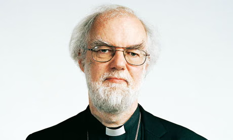
However, a recent visit with a friend re-introduced me to Rowan Williams, who offers not “theology that bites back” but the mystic’s voice: “Consider the lilies. They neither toil nor spin.” Trust God. Let go. This sounds like wisdom—until it sounds like fatalism. Or worse, Islam’s inshallah: whatever will be, will be.

Which is it? Fight for culture or let God do the fighting?

The question feels urgent, binary. Kierkegaard would recognize it immediately—the tyranny of “Either/Or” thinking. Pick a side. You’re either with us or against us.

Rowan Williams—Welsh poet, patristics scholar, former Archbishop of Canterbury—spent a decade frustrating everyone by refusing to choose.

During his 2002-2012 tenure, activists wanted decisive stands. Conservatives wanted tradition defended. Progressives wanted him leading the charge. Everyone wanted a general willing to marshal troops.

Instead, they got a contemplative who wrote poetry, translated fourth-century mystics, and gave maddeningly nuanced answers. When pressed on sexuality debates threatening to split global Anglicanism, he chose patient dialogue over ideological purity. The right called him weak. The left called him complicit.

But Williams wasn’t confused. He was inhabiting the tension rather than resolving it. He learned this from Christianity’s most unlikely revolutionaries—the Desert Fathers.

In his book Silence and Honey Cakes, Williams introduces these strange rebels. When fourth-century Christianity became the empire’s official religion and bishops wore imperial robes, thousands of Christians fled to the Egyptian desert.

These weren’t quietists. They saw that “winning” the culture war meant losing everything that mattered. The empire embraced the church; the church became imperial. To bishops negotiating with emperors, accumulating wealth, defining orthodoxy through political power, the Desert Fathers said: No.

They didn’t storm halls of power or write manifestos. They walked into the wilderness with nothing and sat down.

And from that wilderness, they changed everything.

Here’s what Williams sees: their withdrawal was the most political act imaginable. They weren’t escaping the culture war—they were fighting it on completely different terms.

The empire said power comes from influence, wealth, control. The Desert Fathers built nothing, owned nothing, controlled nothing.

The culture said identity comes from role, status, accomplishments. The Desert Fathers literally forgot their names in silence.

The economy said value equals productivity. The Desert Fathers sat absolutely still for hours, producing nothing, calling it the world’s most important work.

This drove visitors crazy. Pilgrims traveled weeks seeking wisdom, and the hermit would say: “Go, sit in your cell, and your cell will teach you everything.”

It sounds like non-engagement. But Williams argues the opposite: the desert wasn’t retreat from reality—it was the only place to see reality clearly.

The activist impulse runs deep in American Christianity. Save the culture. Win the argument. Build the institution. Doug Wilson’s approach resonates because it feels faithful, muscular. “Faith without works is dead,” right?

But Williams asks: What if all your frantic activity is baptized anxiety? What if your need to “fight for the culture” is actually ego—your need to matter, to win? What if activism is driven not by love but fear—fear of irrelevance, of God not showing up unless you make it happen?

The Desert Fathers called this logismoi—the swirling thoughts driving us, compulsions masquerading as virtues. Until you sit still enough to see these illusions clearly, every “good work” is contaminated by them.

In the desert, they learned apatheia—not apathy, but freedom from reactive passions. Acting from clarity rather than compulsion, love rather than fear, trust rather than control.

This drove Williams’ critics mad. They wanted reaction. He offered contemplation. They wanted tribal certainty. He offered nuanced discernment. They wanted a general. He gave them a monk.

But doesn’t this collapse into Islamic fatalism? If we’re supposed to trust God, why act at all?

Here’s Williams’ crucial synthesis:

The fatalist says: “My actions don’t matter, so why try?” Despair disguised as piety.

The activist says: “Everything depends on me, so I must never rest.” Pride disguised as faithfulness.

The contemplative says: “God is acting, and I get to participate—but the outcome isn’t mine to control.” This is freedom.

Look at Jesus. Forty days in the desert before public ministry. Regular withdrawal sustaining public work. He engaged culture—healing, teaching, confronting power. But he acted from deep rootedness in the Father, from abundance not anxiety.

The night before his arrest, Peter draws a sword. Jesus says: put it away. Not because he’s passive, but because he’s operating from completely different understanding of power. That’s not fatalism. That’s the most radical trust in human history.

Kierkegaard’s Either/Or presents seemingly incompatible life choices: aesthetic or ethical, pleasure or duty. But Kierkegaard knew the title itself is the trap. The mature person doesn’t choose between them; they integrate them at a higher level in the “religious” stage.

Williams does the same with contemplation and action. We must trust and act. Withdraw and engage. Cultivate silence and speak prophetically.

Think of it like breathing. Inhale: contemplation, withdrawal, receiving. Exhale: action, engagement, giving. You can’t live by only inhaling—you’ll burst. You can’t live by only exhaling—you’ll collapse.

The question isn’t calculating the perfect ratio. It’s: Are you rooted deeply enough to engage wisely?

But here’s where Williams’ approach faces its most devastating critique: What about when evil demands immediate action?

Consider the lilies while babies are being aborted? Cultivate silence while DEI policies systematically discriminate? Would Williams have been Churchill or Chamberlain?

Edmund Burke haunts us: “The only thing necessary for the triumph of evil is for good men to do nothing.” Hitler didn’t need more Rowan Williams types—he needed the church to fight.

When Bonhoeffer returned to Germany in 1939, he chose conspiracy and resistance over safe contemplation. When Wilberforce fought the slave trade for decades, he wasn’t told to “consider the lilies.”

So is Williams wrong?

No—but he’s incomplete if we don’t understand what contemplation actually produces.

The Desert Fathers weren’t pacifists—they were the fiercest warriors against evil. But they understood the deepest evils are spiritual, and you can’t fight spiritual battles with carnal weapons. Athanasius, who fought Arianism for decades, learned his theology from Anthony of the desert. The contemplative produced the fighter.

Those silent monks became the theological backbone resisting imperial heresy. When emperors demanded doctrinal compromise, the desert tradition held firm. Their withdrawal gave them clarity and courage to resist.

Contemplation isn’t an alternative to fighting evil—it’s what equips you to fight the right battles in the right way for the right reasons.

The activist who never contemplates will fight—but against what? With what weapons? Driven by what spirit? We’ve seen conservatives become indistinguishable from the left in tactics, spirit, tribalism. They’re fighting like the world fights, which means they’ve already lost.

DEI is evil when it judges people by immutable characteristics rather than character and competence. Fight it. But how? By becoming equally tribal, equally discriminatory—just reversed? That’s not winning; that’s becoming what you oppose.

The pro-life movement’s greatest victories haven’t come from politicians screaming on cable news—they’ve come from crisis pregnancy centers, changed hearts, decades of patient work.

So practically, what does this mean?

First, check your motivations. Is this flowing from prayer or anxiety? From love or ego? Anxious activism burns out or becomes monstrous.

Second, cultivate depth. If your activism isn’t rooted in regular silence, solitude, prayer—it will corrupt you. Bonhoeffer practiced the disciplines even while plotting against Hitler.

Third, embrace the long game. The Desert Fathers planted seeds that wouldn’t flower for generations. Wilberforce fought twenty years before victory.

Fourth, go smaller, deeper, truer. Don’t grasp for cultural dominance. Build communities of alternative practice. The early church didn’t defeat Rome by winning elections—they built a parallel society so compelling the empire converted.

Fifth, know your real enemies. The Desert Fathers’ battles were internal—pride, vainglory, anger. The same spiritual evil producing DEI—pride disguised as compassion—lives in your heart too.

After a decade trying to hold together a fracturing communion, Williams stepped down and returned to teaching, writing, poetry. Some saw defeat. But maybe it was the most desert move of all: releasing the need to control outcomes, trusting God with the church.

Since leaving Canterbury, Williams has written more explicitly about economic justice, climate change, empire. Freed from institutional power, he’s become more pointed. The withdrawal enabled deeper engagement.

The question Williams forces us to face isn’t whether to engage or trust, fight or pray. It’s: From what source are you living?

Are you acting from union with God, or from anxious need to make something happen? Is your engagement an overflow of contemplation, or a substitute for it?

The Desert Fathers fled not because they didn’t care about the world, but because they loved it too much to let empire define what caring looks like.

Williams spent a decade demonstrating you can be deeply engaged while refusing to let the world’s anxiety determine your response. You can lead without grasping. Care without controlling. Act decisively while holding outcomes loosely.

The culture won’t be saved by Christians who trust God so much they do nothing. Nor by Christians who fight so hard they become indistinguishable from every other power-seeking tribe.

It might be saved by communities who’ve been to the desert. Who’ve sat still enough to see their illusions clearly. Who act not from anxiety but abundance. Who fight not from fear but love. Who engage not to win but to witness.

Who trust God enough to act. And act in ways that demonstrate trust.

The Desert Fathers didn’t defeat empire by organizing coalitions. They defeated it by refusing to let it define reality. By living so differently that people traveled hundreds of miles to ask: “How do you have such peace?”

And when pilgrims arrived expecting great wisdom, the hermits would say: “Go sit in your cell, and your cell will teach you everything.”

Maybe that’s exactly what we need to hear.

Not because culture doesn’t need engagement, but because we can’t engage faithfully until we’ve learned to sit still. Until we’ve discovered that God’s kingdom comes not by might nor power, but by a Spirit we can only encounter in silence.

Then—only then—when we speak, we’ll have something worth saying. When we act, we’ll act from depth. When we fight, we’ll fight for the right things in the right ways.

We’ll fight like people who’ve learned to trust. And trust like people free to act.

Which is to say: we’ll breathe. In and out. Contemplation and action. Desert and city.

Both. And. Not either. Or.

Maybe the way forward isn’t choosing between the culture warrior and the contemplative. It’s becoming the kind of person who’s been silent enough to have something worth saying when they speak.

November 10, 2025 (updated November 10, 2025) By Tim Booher 0 Comments

Personal Projects & Interests

Reformed Christian Perspective on Israel and Modern Judaism

Some American Christians are rethinking what they believe about Israel and Judaism. Shifting geopolitical realities, rising tensions both domestically and internationally, and increasingly polarized discourse have forced questions that have been long settled for me. But before we can answer “What should Christians think about Jews?”, we need to untangle what we’re actually talking about.

We can call something “Jewish”, when it functions as at least five different categories that we habitually collapse into one:

Ethnicity: Genetic descent from Abraham through Isaac and Jacob
Culture: Rich literary and intellectual traditions, distinctive languages (Yiddish, Ladino, Judeo-Arabic), cuisine and foodways, music (klezmer, liturgical, contemporary), art and cinema, philosophical contributions, scientific achievements, centuries of diaspora experience, humor and storytelling traditions, family and community practices, distinct historical memory and commemoration
Faith: Religious belief and practice ranging from secular to ultra-Orthodox
Geopolitics: The modern State of Israel and Middle Eastern policy
Theology: God’s covenant relationship with His chosen people

And within the category of faith alone, “Judaism” spans an enormous spectrum. Reform Jews may not believe in a personal God. Conservative Jews navigate tradition and modernity. Modern Orthodox professionals may study Talmud daily and some ultra-Orthodox communities reject Zionism and don’t recognize the State of Israel. Many friends are secular Jews who identify culturally but not religiously. Even among the religiously observant, there are vast differences in how they relate to foundational texts: Torah (the five books of Moses), Nevi’im (the Prophets), Ketuvim (the Writings), the Talmud (rabbinic discussions and legal interpretations), Midrash (interpretive commentaries), Kabbalah (mystical traditions), and countless generations of rabbinical responsa. Some communities prioritize halakhic (legal) study, others emphasize ethical teachings, still others focus on mystical experience or philosophical theology.

When we ask “What should the Christian posture be toward Jews?” which Judaism are we discussing? The Hasidic community in Brooklyn? The Reform temple down the street? The Israeli soldier? The Hollywood producer? The Talmud scholar? These aren’t interchangeable categories, and our theology must be precise enough to account for these distinctions; not just in what we believe, but in how we relate, engage, and bear witness.

The confusion isn’t just academic. When we lump together ethnicity, faith, culture, and geopolitics, we end up with theological frameworks that can’t distinguish between critique of Israeli policy, rejection of Talmudic tradition, and hatred of Jewish people. We need to disentangle these threads before we can think biblically about any of them.

In the recent words of Stephen Wise, “Jews get to define Judaism, others get to decide if they accept us as we see ourselves”. That’s fair. My answer then of Who and What is provided by the manifold conversations I’ve had with the people who practice their Jewish faith. For me that means two groups: secular Jews largely in military, tech and/or business and faithful religious Jews I know largely through the classroom or conservative political affiliations.

For the purpose of this post, I’m going to assume we are talking about the theological core and shared beliefs of the Jewish faith today as understood through my personal relationships and a bit of reading.

The Biblical Framework or What Christian Scripture Actually Says

Paul’s treatment of Israel in Romans 11 provides the definitive framework for Reformed thinking about Judaism. He describes a remnant chosen by grace (11:5), not wholesale abandonment but divine preservation. He speaks of partial hardening, not total rejection (11:25) Israel’s blindness is temporary and purposeful, not permanent apostasy. Most remarkably, Paul uses present tense: they are “beloved for the sake of their forefathers” (11:28), not were beloved. God’s love for Israel continues in the present, not just the past. The gifts and calling of God are irrevocable (11:29), God doesn’t break covenants, even when His people stumble.

This language is incompatible with viewing Judaism as a pagan or demonic religion. Paul explicitly warns Gentile believers against arrogance toward the natural branches (11:18-22). If post-Temple Judaism were intrinsically demonic, Paul’s entire argument collapses.

Revelation’s Vision: Israel in God’s Future

Revelation’s vision of the end times offers a striking confirmation of Israel’s enduring place in God’s purposes. When the Apostle John sees the future unfold, he doesn’t witness Israel’s erasure or replacement, he sees their distinct preservation. The 144,000 sealed from the twelve tribes of Israel appear in Revelation 7 and 14, not as a metaphor emptied of ethnic meaning, but as testimony to God’s faithfulness to His covenant people. The New Jerusalem itself bears witness to this continuity and its twelve gates are named for the twelve tribes, inscribed into the architecture of God’s eternal city (Revelation 21:12). Even the apocalyptic measuring of the temple and those who worship there (Revelation 11:1-2) maintains Israel’s specific identity in God’s final purposes. Whether we read these passages literally or symbolically, the theological point remains unshakeable, namely that God has not abandoned His covenant relationship with Israel as a people.

This biblical vision helps us understand what “demonic” actually means in Scripture’s categories. The word isn’t a catch-all for “things Christians disagree with” it has specific, defined boundaries. Scripture reserves “demonic” language for idol worship and service to false gods (Deuteronomy 32:17; 1 Corinthians 10:20), conscious opposition to Christ as the Antichrist spirit (1 John 2:22), and occult practices and divination explicitly condemned in the Law (Leviticus 19:31; Deuteronomy 18:10-12). These are clear categories with clear markers.

Rabbinic Judaism, even in its tragic rejection of Jesus as Messiah, doesn’t fit these categories. Jews continue to worship the Creator God of Abraham, Isaac, and Jacob the same God Christians worship, though they cannot see His full revelation in Christ. They maintain the Hebrew Scriptures as authoritative and binding, the very Scriptures that testify to Jesus. They order their lives around prayer, repentance, and holiness, seeking to live before the God who gave Torah at Sinai. They faithfully preserve the Sabbath, the biblical festivals, and the covenant markers that God Himself instituted. This isn’t apostasy to demons, it’s spiritual blindness to the fulfillment that has come.

The center of gravity remains the God of Israel, not Molech or Baal. This is blindness to fulfillment, not apostasy to paganism.

The Talmud Question: Corruption vs. Apostasy

One argument made recently (by folks in my hometown of Fort Worth) is that a careful reading of the Talmud reveals a wholly corrupted Jewish faith that ancient Jews wouldn’t recognize. But this claim requires significant qualification. First, not all Jews hold the Talmud (the oral tradition) on par with the written tradition. The Jewish world is far more diverse in its relationship to rabbinic texts than many critics acknowledge.

The Talmud does present legitimate concerns for Christians. It can obscure grace under layers of legal reasoning, making the encounter with God’s mercy harder to see. Some passages reflect hostility toward Christianity, shaped by centuries of conflict and persecution. It solidifies a system that, without Christ, cannot ultimately save. Certain mystical traditions drift toward problematic territory that should give us pause. These are real issues that deserve honest theological engagement.

But we must be careful not to mistake corruption for apostasy, or development for departure. The Talmud is fundamentally an in-house Jewish attempt to order life before the God of Israel according to Torah. It’s not a manual for worshiping a different deity. It’s rabbinic Judaism wrestling with the question: How do we remain faithful to the covenant when the Temple is destroyed and the priesthood scattered? This distinction matters enormously when we’re trying to assess whether we’re dealing with blindness to fulfillment or apostasy to demons.

Consider Jesus’ own approach to Pharisaic tradition, which became the foundation for what evolved into rabbinic Judaism. He blasts their additions and burdens in Matthew 23, calling out their hypocrisy and legalistic distortions with searing clarity. Yet in the same breath, He acknowledges “they sit in Moses’ seat,” recognizing their legitimate authority to interpret Torah. He debates within the framework of Jewish tradition, not as an outsider confronting a foreign religion. This is the posture of a reformer calling His people back to covenant faithfulness, not a missionary encountering paganism.

What continues from ancient Judaism to its modern expression tells us something crucial. The same God remains central: the Shema, “Hear, O Israel: the LORD our God, the LORD is one,” is still prayed daily. The same Scriptures are read, studied, and revered. The same covenant markers: circumcision, Sabbath, dietary laws structure Jewish life. The same fundamental hope persists, even if Messianic expectation is understood differently. Many of the same prayers are still recited, some dating back to Temple times. This isn’t wholesale replacement; it’s recognizable continuity.

What changed after the destruction of the Temple represents adaptation within tradition rather than abandonment of it. Temple sacrifice was replaced by prayer and study, following the prophetic principle that God desires mercy more than sacrifice. Priestly authority gave way to rabbinic interpretation as the community needed new leadership structures. Messianic hope was deferred rather than recognized in Jesus a tragic blindness, but still hope directed toward the God of Abraham. The oral Torah was codified in Talmud and Midrash to preserve what had been transmitted verbally for generations. Theological emphasis shifted from sacrifice to ethics and law as the community sought ways to maintain covenant relationship without the Temple system.

This is development within the same tradition, not the creation of a new religion. A first-century Pharisee, transported to a modern Orthodox synagogue, would recognize far more than he’d find foreign. He would hear familiar prayers, see familiar rituals, recognize the Torah scroll and its reverent treatment. He might be shocked by some theological developments, puzzled by certain innovations, but he wouldn’t think he’d stumbled into a temple of Baal or Molech. The center of gravity, the God of Israel, the authority of Scripture, the covenant relationship, remains recognizably continuous.

Contemporary Jewish belief spans an enormous spectrum, and any analysis that treats it as monolithic fails before it begins.

Within contemporary Judaism, the diversity of belief and practice is staggering. Ultra-Orthodox communities structure entire lives around intensive Talmud study and strict halakhic observance, often living in insular neighborhoods where religious law governs every detail from sunrise to sunset. Modern Orthodox Jews navigate a different balance, engaging Torah deeply while participating fully in modern professional and cultural life: doctors and lawyers who spend their evenings studying ancient texts. Conservative Judaism attempts to honor historical tradition while applying critical scholarship to its sources, creating communities that look traditional but think historically. Reform Judaism emphasizes ethical monotheism over ritual observance, seeing Judaism primarily as a moral framework rather than a legal system. And millions of secular Jews maintain strong cultural identity, celebrating Passover, mourning the Holocaust, supporting Israel, while holding no particular religious beliefs at all.

The claim that “all rabbinic Jews reject God dwelling with man” reveals a fundamental unfamiliarity with Jewish sources and practice. The concept of the Shekhinah, God’s divine presence dwelling among His people, remains absolutely central to traditional Jewish thought across denominations. Every synagogue service explicitly invokes God’s presence. Hasidic traditions speak constantly of encountering the divine in everyday life. Jewish mysticism, from medieval Kabbalah to modern Hasidism, emphasizes divine immanence with an intensity that would surprise critics. Contemporary Jewish philosophers like Abraham Joshua Heschel and Martin Buber have written profoundly about divine-human encounter. To claim Judaism categorically denies God’s presence is simply false.

When Christians carelessly label Judaism “demonic,” a cascade of consequences follows that extends far beyond theological error. We forget that our own Scriptures emerged from Jewish scribes, that our Savior lived as a Torah-observant Jew, that our first apostles were all Jewish believers who saw Jesus as Messiah, not as founder of a new religion. We undermine Paul’s carefully constructed argument in Romans about Israel’s ongoing significance in God’s purposes. We create space for actual antisemites to claim Christian validation for their hatred. We destroy any credible witness to Jewish communities, who would listen to someone who’s already declared them demonic? And most dangerously, we align ourselves with ideological movements that have historically led to persecution and atrocity.

Luther’s Warning: When Evangelical Frustration Becomes Genocidal Blueprint

The Reformed tradition must reckon honestly with how this trajectory has played out in our own history. Martin Luther provides the most sobering example, and for those of us who love Luther, who have been shaped by his theological courage, his biblical insight, his unwavering commitment to justification by faith alone, this reckoning is painful. I count myself among Luther’s admirers. His stand at Worms, his translation of Scripture, his hymns, his exposition of Galatians, these have nourished my faith and the faith of millions. Which makes his writings on the Jews not just historically troubling but personally grievous. We cannot love Luther rightly without lamenting this aspect of his legacy deeply.

In his earlier years, Luther criticized the Catholic Church’s treatment of Jews and held hope for mass Jewish conversion once the Gospel was freed from papal corruption. His 1523 work “That Jesus Christ Was Born a Jew” showed genuine concern for Jewish evangelism and criticized Christian mistreatment.

But when Jews failed to convert in the numbers Luther anticipated, his frustration curdled into something far darker. By 1543, Luther published “On the Jews and Their Lies,” a document so venomous that the Nazis would later display it at Nuremberg rallies. Luther called for burning synagogues, destroying Jewish homes, confiscating prayer books and Talmudic writings, forbidding rabbis from teaching, abolishing safe conduct for Jews on highways, banning usury, and forcing Jews into manual labor. His theological justification? That the Jews’ rejection of Christ proved them to be children of the devil, their synagogues “a den of devils,” their worship demonic.

The progression is instructive and terrifying. Luther began with orthodox Christian conviction, faith in Christ is necessary for salvation. He added urgent evangelistic hope, surely Jews will recognize their Messiah when the Gospel is clearly preached. When reality disappointed, Jews remained unconvinced, theological frustration transmuted into demonization. And demonization inevitably produced calls for persecution. If Jews are demonic, if their worship is satanic, if their very presence pollutes Christian society, then violence becomes not just permissible but pious.

Four centuries later, Nazi propagandists didn’t have to invent Christian antisemitism, they simply dusted off Luther and gave his recommendations modern implementation. When Kristallnacht came on this day (9 Nov) in 1938, synagogues burned across Germany on November 9th, Martin Luther’s birthday. The switch can happen: righteous evangelical urgency can become dark ethnic hatred; theological conviction can become demonization.

The lesson isn’t that we should soft-pedal the Gospel or pretend Jewish rejection of Christ doesn’t matter. Luther was right that Jesus is the only way to salvation. He was right that post-Temple Judaism cannot save. He was catastrophically, damnably wrong in moving from “Jews need Christ” to “Jews are demonic” to “Jews should be persecuted.” The slide from the first to the second happens when we lose Paul’s nuance in Romans 11. The slide from the second to the third is inevitable, it’s simply a matter of time and political opportunity.

A faithful Reformed perspective maintains what might seem like contradictory truths, holding them in tension as Scripture does. Salvation is in Christ alone, any religious system that rejects Jesus cannot ultimately save. Judaism without Christ remains incomplete and broken, with the veil over Moses still unlifted, as Paul describes in 2 Corinthians. Yet simultaneously, Israel remains beloved for the sake of the patriarchs, their gifts and calling irrevocable. The root of the olive tree is holy, and we Gentile believers are grafted into Israel’s story, not the reverse. And crucially for our historical moment, antisemitism, the hatred of Jewish people, stands in direct opposition to God’s purposes and the Gospel itself. These truths don’t contradict; they complete each other.

This framework allows us to evangelize Jewish people with urgency and love, understanding that faith in Christ is essential for salvation while recognizing we’re speaking to those who already know the God of Abraham. It enables us to oppose antisemitism wherever it emerges, whether in progressive spaces that cloak hatred in anti-Zionism or in conservative circles that traffic in conspiracy theories. We can appreciate Judaism’s remarkable preservation of Scripture and its ongoing witness to monotheism, even while maintaining that this witness remains incomplete without Christ. Most importantly, we can hold theological clarity without resorting to demonization, recognizing the profound mystery of Israel’s future restoration that Paul describes in Romans 11:25-26.

These theological commitments have concrete implications for how Christians engage the world today. In theological discussion, we must reject the simplistic “Judaism is demonic” rhetoric that has gained traction in some corners of the internet and most alarmingly in the Church. The distinction between spiritual blindness and pagan apostasy isn’t semantic hairsplitting, it’s the difference between biblical fidelity and dangerous error. Before making sweeping pronouncements about Judaism, Christians should immerse themselves in Romans 9-11, where Paul wrestles with these very questions with far more nuance than most contemporary commentators manage.

In political engagement, the stakes are even higher. Christians must refuse to platform antisemites, regardless of how much we might agree with their positions on other issues. Supporting Israel’s right to exist doesn’t require blind endorsement of every policy decision, just as loving Jewish neighbors doesn’t mean abandoning theological convictions. But we must be clear, theological disagreement never justifies persecution, marginalization, or hatred. When antisemitism appears in progressive spaces or conservative ones, Christians must call it out with equal vigor.

The most transformative engagement, though, happens in personal relationships. Building genuine friendships with Jewish neighbors, learning about Judaism from practicing Jews rather than plucking random passages from the Talmud to construct caricatures, sharing the Gospel with love rather than contempt, these ordinary interactions matter more than grand theological pronouncements. Christians can celebrate what Judaism has faithfully preserved through centuries of persecution while pointing to its fulfillment in Christ. We can study together, disagree deeply, and still recognize our shared heritage in the God of Abraham, Isaac, and Jacob.

Church teaching bears special responsibility in this moment. Pastors must preach the whole counsel of Scripture on Israel, including the difficult passages that don’t fit neatly into either supersessionist or dispensationalist categories. Replacement theology that erases Israel’s ongoing significance contradicts Paul’s explicit teaching, but so does any framework that ignores Judaism’s tragic blindness to its own Messiah. Churches must teach Christian history honestly, including the shameful legacy of Christian antisemitism that provided theological cover for persecution and genocide. Only by facing this history squarely can we prepare our congregations to engage Jewish friends, neighbors, and colleagues with both theological clarity and genuine love.

To declare Judaism “demonic” is to saw off the branch we’re sitting on. Christianity emerges from Judaism, fulfills Judaism’s hopes, and shares Judaism’s Scriptures. Our Savior was a Torah-observant Jew who prayed the Shema, kept the Sabbath, and celebrated Passover. The apostles were Jews who saw Jesus as Israel’s Messiah, not a foreign deity. Yes, modern Judaism’s rejection of Jesus is spiritually fatal. Yes, the Talmudic tradition includes problematic elements. Yes, we must evangelize Jewish people with urgency. But we must do so recognizing what Paul knew, this is family business. We’re dealing with elder brothers who can’t see the family resemblance in the One they reject, not strangers worshiping foreign gods. They are “enemies for your sake” but “beloved for the sake of the fathers” (Romans 11:28).

The Reformed tradition at its best provides the clarity our moment demands. Unwavering commitment to salvation in Christ alone, coupled with deep respect for God’s irrevocable calling of Israel. This isn’t theological compromise, it’s biblical fidelity. The way forward isn’t through demonization but through faithful witness, proclaiming Christ as the fulfillment of Israel’s hope while standing firmly against those who would harm the people through whom salvation came to the world. This is the Reformed position, the biblical position, and the only position that takes seriously both the Gospel’s exclusivity and God’s covenant faithfulness. As Paul concludes his meditation on Israel’s mystery, “Oh, the depth of the riches both of the wisdom and knowledge of God! How unsearchable are His judgments and His ways past finding out!” (Romans 11:33). That humility, not internet boldness or reactionary provocations, should mark our engagement with the mystery of Israel and the Jewish people.

November 9, 2025 (updated July 11, 2026) By Tim Booher One Comment

Personal Projects & Interests

The Data Doesn’t Lie: How 266 Runs Revealed The Truth About My Marathon Goal

For the BMW Marathon in Dallas, I’m targeting 7:30/mile pace—a 3:16:45 finish, what training plan should I follow from today? Work has been insane stressful, and has destroyed my training. Can AI help me here?

My long runs felt good at that pace for 8-10 miles, so I thought I was on track. I’m always testing to see how much I can do myself and I’m curious to use AI to coach me. AI isn’t useful without the right data, so I analyzed 266 runs from the past two years to build a good training plan.

The most recent data is the most important, so it was important that I took note of my run this morning. I ran a half marathon at 8:10 average pace with a heart rate of 137-148 bpm—very easy aerobic effort. I finished the last two miles at 7:42 and 7:49 pace.

Here’s what 266 runs over two years revealed:

DISTANCE RANGE	RUNS	AVERAGE PACE	BEST PACE	PATTERN
3-4 miles	92	8:14	6:44	Speed is there!
6-7 miles	31	8:25	7:23	Solid training pace
10-11 miles	8	8:11	7:47	Sub-8:00 capability proven
13-14 miles	3	7:48	7:53	THE SWEET SPOT
14-15 miles	2	7:54	7:41	Strong mid-distance
16-17 miles	2	8:26	8:20	Starting to fade
18-19 miles	2	8:11	7:44	Inconsistent
20+ miles	5	8:54	8:00	THE PROBLEM

The pattern was clear: 13-14 mile average of 7:48 versus 20+ mile average of 8:32. A 44-second-per-mile dropoff. My best 20+ mile run: 8:00 pace. Still 30 seconds slower than goal. My average 20+ mile run: 8:32 pace. A 1:02/mile gap to close. But this morning’s half marathon told a different story. I ran 13.1 miles at low heart rate (137-148 bpm) and finished strong at 7:42-7:49 pace. “Very easy,” I noted afterward. “Could have done a lot more.” This suggests my aerobic base is much better than the historical 8:32 suggests. That average likely came from poor pacing on long runs, not lack of fitness.

My 3-4 mile best pace: 6:26. That’s 1:04 faster than my marathon goal. The problem isn’t speed—it’s extending that speed over distance. The gap: extending my 7:48 pace from 13-14 miles to 20+ miles, then racing smart for 26.2 miles. When you define it that specifically, you can build a plan to address it.

The dropoff from 7:48 pace (13-14 miles) to 8:32 pace (20+ miles) isn’t random—it’s physiological. Research on elite marathoners shows that even well-trained runners deplete muscle glycogen stores significantly after 90-120 minutes at marathon pace. For me, 13-14 miles at 7:48 takes about 1:47—right in the window where glycogen runs low. When I push to 20 miles without proper fueling and without training my body to use fat efficiently, I hit the metabolic wall. But fuel isn’t the only issue. My legs simply aren’t conditioned for the distance.

By “legs aren’t ready,” I mean muscular endurance breaks down, neuromuscular efficiency degrades, and form deteriorates. The quads that fire smoothly at mile 10 are misfiring by mile 18. The signal from brain to muscle becomes less crisp. Motor unit recruitment—the coordinated firing of muscle fibers—gets sloppy. I’m sending the same “run at 7:45 pace” command, but my legs execute it as 8:30 pace. Meanwhile, small biomechanical breakdowns compound: hip drops slightly, stride shortens, each foot strike becomes less efficient. Running 20 miles means roughly 30,000 foot strikes. If I haven’t progressively trained my legs to absorb that cumulative pounding, my body literally slows me down to prevent injury.

Studies on elite marathon training show successful marathoners spend 74% of their training volume at easy intensity (Zone 1-2) because it builds aerobic capacity without accumulating neuromuscular fatigue. My data suggests I was probably running too many miles too hard, accumulating fatigue faster than I could recover—especially at 48. Research on masters athletes shows recovery takes 10-20% longer after age 40. Some coaches recommend 10-12 day training cycles for older athletes instead of traditional 7-day cycles, allowing more space between hard efforts. If I’m not recovering fully before the next quality session, my 20+ mile pace suffers even more than it would for a younger runner.

There’s also cardiovascular drift to consider. During prolonged running, cardiac output gradually decreases while heart rate increases to compensate. This is more pronounced at higher intensities. If I’m running long runs at or near race pace (7:30-7:50), I’m experiencing significant cardiovascular drift by mile 15-18. The effort to maintain pace increases exponentially. My 20+ mile pace of 8:32 might simply reflect the point where my cardiovascular system says “enough.”

My training strategy alternates run days with bike days—typically 18-28 miles at 15-18 mph. Research shows that cycling can maintain aerobic fitness while reducing impact stress, with one mile of running equaling approximately three miles of cycling for cardiovascular equivalence. This means my weekly aerobic load is higher than running mileage suggests: 45 miles running plus 85 miles cycling equals roughly 73 “running equivalent” miles per week. The cycling protects my legs while maintaining cardiovascular fitness—smart training at 48. But it also means my running-specific adaptations (neuromuscular patterns, impact tolerance, glycogen depletion management) might be underdeveloped relative to my aerobic capacity.

The data reveals a specific problem: I have speed (6:26 for 3-4 miles), good mid-distance endurance (7:48 for 13-14 miles), and strong aerobic fitness (cycling adds volume). But I haven’t trained the specific adaptation of holding sub-8:00 pace beyond 14 miles. This isn’t a fitness problem—it’s a specificity problem. The solution isn’t to run more miles. It’s to progressively extend the distance at which I can hold my proven 7:48 pace, while managing fatigue and recovery as a 48-year-old athlete.

Traditional marathon training plans prescribe long runs at “easy pace” or 30-60 seconds slower than race pace. That builds aerobic base, but it doesn’t address my specific limitation: I need to teach my body to hold quality pace for progressively longer distances.

This morning’s half marathon changes the starting point. Instead of beginning conservatively at 16 miles, I can start more aggressively at 18 miles next Saturday. The plan builds from there: 18 miles at 7:50 average pace (two miles easy warmup, 14 miles at 7:45-7:50, two miles easy cooldown). The goal is simple—extend this morning’s easy 13.1-mile effort to 14 quality miles. Week two pushes to 20 miles at 7:45 average, tackling my historical problem distance at a pace 47 seconds per mile faster than my 8:32 average. Week three peaks at 22 miles averaging 7:40 pace—the breakthrough workout that proves I can hold sub-7:40 pace for 18 continuous miles.

After peaking, the volume drops but the intensity holds. Week four: 16 miles at 7:35 average with 12 miles at race pace (7:30-7:35). Week five adjusts for Thanksgiving with 14 miles at 7:35. Week six is the dress rehearsal: 10 miles with six at 7:25-7:30 pace, confirming goal pace is ready. The progression is deliberate—each week either extends distance or drops pace by five seconds per mile, allowing physiological adaptation without overwhelming the system. Elite marathon training research supports this approach: progressive overload with strategic recovery.

Tuesday speedwork leverages my natural speed. My best 3-4 mile pace is 6:26—more than a minute per mile faster than marathon goal pace. Research consistently shows that running intervals 30-60 seconds faster than marathon pace improves race performance by increasing VO2 max, improving running economy, and creating a “speed reserve” that makes race pace feel controlled.

The plan starts with 8×800 meters at 6:30 pace (3:15 per repeat) with 90-second recovery jogs—establishing that I can run fast repeatedly. Week two builds to 10×800 at the same pace. Week three shifts to marathon-specific longer intervals: 6×1200 meters at 6:40 pace. Week four is a six-mile tempo run at 7:10-7:15 pace—faster than race pace, sustained effort. The final speedwork comes in week five: 6×800 at 6:25 pace for sharpness, not volume. Running 6:30 pace in workouts creates a one-minute-per-mile speed reserve over my 7:30 goal. Analysis of 92 sub-elite marathon training plans found successful programs include 5-15% high-intensity training. My Tuesday sessions provide exactly this stimulus.

At 48, recovery determines whether I arrive at race day peaked or exhausted. Complete rest days come every five to six days—no running, no cross-training, just rest. Easy runs stay at 6-7 miles at 8:20-8:30 pace, conversational effort that builds aerobic capacity without adding fatigue. Bike days alternate with run days: recovery rides of 18-22 miles at 15 mph with high cadence and low resistance, or moderate rides of 22-28 miles at 16 mph for steady aerobic work. The cycling maintains cardiovascular fitness and increases blood flow to running muscles while reducing impact stress. Research on masters runners consistently emphasizes that recovery adaptations—not just training adaptations—determine race day performance for athletes over 40.

Fueling practice matters as much as the miles themselves. My data shows pace dropping significantly after 90-120 minutes, suggesting glycogen depletion. Case studies on elite marathoners found optimal race-day fueling to be 60 grams of carbohydrate per hour, delivered as 15 grams every 15 minutes in a 10% carbohydrate solution. I need to practice this in training, not just on race day. Every long run over 90 minutes becomes a fueling rehearsal at goal pace.

This morning’s half marathon rewrites the race plan. I ran 13.1 miles at low heart rate (137-148 bpm), averaging 8:10 for the first 11 miles before closing the last two at 7:42 and 7:49 pace. My note afterward: “very easy, could have done a lot more.” That performance suggests my aerobic base is significantly better than my historical 8:32 average for 20+ miles indicates. That average likely came from poor pacing on long runs, not lack of fitness.

The conservative approach mirrors this morning’s pattern: controlled start, gradual build, strong finish. Miles 1-10 at 7:30-7:35 pace—just like this morning’s easy start—predicted split of 1:15:00 to 1:16:40. It will feel easy, almost too easy. The temptation will be to push harder. Don’t. Miles 11-20 settle into goal pace range at 7:28-7:32, predicted split of 1:15:00 to 1:16:00. This is half-marathon distance, and my data proves I can hold 7:48 pace for 13-14 miles. Running 7:30-7:35 is only 13-23 seconds per mile faster—controlled and sustainable. Miles 21-26.2 finish strong at 7:25-7:30 pace, just like this morning’s close. Predicted split: 38:45 to 39:00. Total projected finish: 3:15:00 to 3:16:45.

The aggressive approach—even 7:30 splits from mile one for a 3:16:45 finish—only makes sense if week three’s 22-mile peak run at 7:40 average feels as easy as this morning’s half marathon felt, if weather is perfect (50-55°F, low humidity, no wind), if taper goes flawlessly, and if I wake up on race day feeling exceptional. Otherwise, the conservative negative split strategy is smarter.

Three scenarios, all representing massive improvement over historical data. Best case: 3:15:00-3:16:00, requiring perfect execution of the conservative strategy and this morning’s negative split pattern. Probability: 45 percent, up significantly after this morning’s performance. Realistic: 3:16:00-3:17:00, solid execution with maybe imperfect conditions. Probability: 40 percent. Solid: 3:17:00-3:18:30, good race with slight fade or challenging conditions. Probability: 15 percent.

All three outcomes crush the historical 8:32 pace for 20+ miles. All three are victories. The goal isn’t to cling to 7:30 pace at all costs—it’s to run the smartest race possible given training data and this morning’s proof that the aerobic base is there.

I thought I was running long runs at 7:30 pace. The data showed 7:48 for 13-14 miles and 8:32 for 20+ miles. Memory is selective. Data isn’t.

But this morning’s half marathon revealed something the historical data missed: I ran 13.1 miles at a heart rate of 137-148 bpm—easy aerobic effort—and finished strong at 7:42 and 7:49 pace. Afterward, I noted “very easy, could have done a lot more.” That 8:32 average for 20+ miles wasn’t about fitness—it was about pacing. I’d been going out too hard and fading. The aerobic base is better than the numbers suggested.

The limitation isn’t speed—my best 3-4 mile pace is 6:26. It’s not aerobic fitness—the cycling adds significant volume and this morning proved the engine is strong. The gap is specificity: I haven’t trained to hold quality pace beyond 14 miles. At 48, I need more recovery than I did at 35. Research shows masters athletes need 10-20% more recovery time. The alternating run-bike schedule isn’t a compromise—it’s smart training that keeps me healthy enough to execute the progressive long runs that will close the gap.

Seven weeks to race day. Progressive long runs build from 18 to 22 miles at progressively faster paces. Tuesday speedwork at 6:30 pace creates a one-minute-per-mile reserve over goal pace. Complete rest every five to six days. Race strategy mirrors this morning’s pattern: controlled start, build into goal pace, finish strong.

Will I hit 3:16:45? Good chance—this morning proved the base is there. Will I run 3:16:00-3:17:00? More likely. Either way, it’s significantly faster than 8:32. The data showed the problem. This morning showed the solution. Now execute.

RESEARCH REFERENCES

Stellingwerff, T. (2012). “Case Study: Nutrition and Training Periodization in
Three Elite Marathon Runners.” International Journal of Sport Nutrition and
Exercise Metabolism, 22(5), 392-400.
Sports Medicine – Open (2024). “Quantitative Analysis of 92 12-Week Sub-elite
Marathon Training Plans.”
Tanaka, H. (1994). “Effects of cross-training. Transfer of training effects on
VO2max between cycling, running and swimming.” Sports Medicine, 18(5), 330-339.
Runner’s World / Marathon Training Academy (2024-2025). “Marathon Training After 50”

Research on masters athlete adaptations and recovery needs.

Haugen, T., et al. (2019). “The Training and Development of Elite Sprint Performance: an Integration of Scientific and Best Practice Literature.” Sports Medicine – Open.

October 25, 2025 (updated October 26, 2025) By Tim Booher One Comment

Personal Projects & Interests

Fixing the inlet on my Ryobi Pressure Washer

Some posts I write to inform others of cool stuff. Others posts I write to save someone else time when they google. This post is just a story of frustration, written to look like the second example. You have been warned.

Several years ago, I bought this pressure washer and then let it sit unused for far too long—a bad move. The Ryobi RY80940B, powered by a Honda GCV190 engine, delivers 3,100 PSI at approximately 2.5 GPM, more than enough force for serious cleaning but also enough to punish neglected hardware. For anyone working on one of these, the operating manual is available here: Ryobi RY80940B Service Manual (PDF).

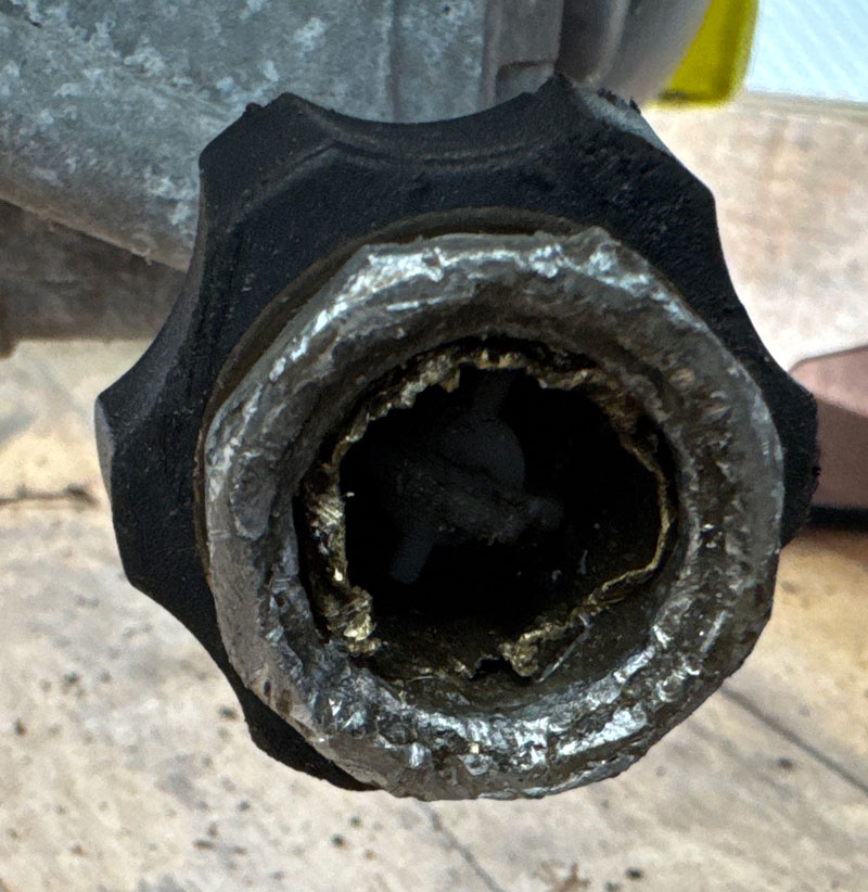
When I finally tried to remove the hose, the metal fitting was stuck. The smart thing would have been to leave the hose stuck in there forever. I didn’t do that. I wanted to get the old hose out and, well, I’m an arrogant engineer and this was a battle of wills not of wits. I’ve spent the better part of an afternoon fighting with a broken brass fitting fused inside the outlet coupler of my Ryobi RY80940B pressure washer. What should have been a simple hose replacement turned into a problem. The brass insert from the old high-pressure hose sheared off cleanly, leaving a ring of corroded metal wedged inside the plastic spindle. I tried everything — prying, tapping, a bolt extractor — but the brass just spun or smeared instead of breaking free.

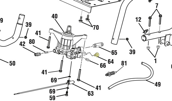
Eventually, I realized I was wasting time trying to rescue a part that costs less than lunch. The black collar that covers the quick-connect doesn’t unscrew; it slides over a spring and bearing set. Once you see the parts diagram for this model, it’s obvious the spindle (part #642058001) and collar (part #310993003) are meant to be replaced together.

Per the service manual, I first tried an 8 mm hex key to back out the fitting, but it immediately began to strip, producing nothing but a rain of metal shavings.

After exhausting every polite method of extraction, I escalated. Since I knew the brass and aluminum had fused completely, I cut most of the seized coupler off with an angle grinder, then used diagonal cutters to peel the remaining sleeve away from the spindle. With the bulk removed, I applied heat from a torch, clamped a pair of vice grips onto what was left, and added a four-foot cheater bar for leverage. The grips slipped off more than once, but eventually I felt the faint give of motion—the threads finally broke free. Sometimes the “fix” isn’t surgical precision; it’s controlled brutality, executed carefully enough not to destroy the surrounding parts.

Because this took so much work. I’m going to show you two pictures.

Tech Details

So what happened here? The failure wasn’t merely mechanical — it was electrochemical and thermomechanical. The brass hose insert (nominally Cu–Zn alloy, ≈ $Cu_{60}Zn_{40}$) had been pressed into a steel spindle (Fe–C alloy with minor Mn, Si). Over years of intermittent water exposure, this dissimilar-metal couple set up a galvanic cell with the water acting as electrolyte. Brass is more noble than steel in the galvanic series:

$$E^\circ_{\text{Cu}^{2+}/\text{Cu}} = +0.337\text{ V}, \quad E^\circ_{\text{Fe}^{2+}/\text{Fe}} = -0.440\text{ V} $$

The potential difference,

$$\Delta E = E_{\text{cathode}} – E_{\text{anode}} \approx 0.777\text{ V},$$

was sufficient to drive anodic dissolution of iron and the formation of iron oxides/hydroxides.

The local electrochemical reactions were:

Anode (steel):

$$\text{Fe} \rightarrow \text{Fe}^{2+} + 2e^-$$

Cathode (brass surface):

$$\text{O}_2 + 2H_2O + 4e^- \rightarrow 4OH^-$$

The resulting $Fe(OH)_2$ and $Fe_2O_3$ corrosion products expanded volumetrically, wedging the interface tighter. The growth strain of oxide formation can be expressed as:

$$\varepsilon_v = \frac{V_{\text{oxide}} – V_{\text{metal}}}{V_{\text{metal}}}$$

For iron oxides, $\varepsilon_v \approx 1.9$, meaning nearly a doubling in volume. This expansion induced radial compressive stress at the interface:

$$\sigma_r = \frac{E \, \varepsilon_v}{1 – \nu}$$

With $E_{\text{Fe}} \approx 210\,\text{GPa}$ and $\nu \approx 0.3$, localized stresses easily exceeded hundreds of MPa, enough to plastically deform the surrounding brass and produce microscopic cold-welding through diffusion and oxide bridging.

At the same time, dezincification occurred in the brass:

$$\text{CuZn} \rightarrow \text{Cu} + \text{Zn}^{2+}$$

leaving a porous copper-rich layer with high surface energy. Under compression and mild heat cycling, solid-state diffusion across the Cu–Fe interface promoted the formation of intermetallic compounds such as $CuFe_2$ or $Fe_3Zn_{10}$, effectively brazing the two metals together.

The end state was a compound joint bonded both by corrosion-product expansion and diffusion adhesion — a quasi-metallurgical weld. The torque required to shear it loose later had to exceed the yield strength of both alloys plus the adhesion energy of the oxide layer:

$$\tau_{\text{break}} \ge \frac{\sigma_y A + \gamma_{\text{adh}}}{r}$$

where $\sigma_y$ is the yield stress, A the contact area, $\gamma_{\text{adh}}$ the oxide interfacial energy, and r the effective radius. I estimate I needed breakaway torque of in the neighborhood of 80–160 N·m, danger close to the ~200-250 N·m that will break a Grade 8.8 M16 bolt — and this was a thin walled threaded tube. The geometry also doesn’t help. Since brass (CuZn) was threaded into the aluminum/steel pump body at M16 scale, the fine 1.5 mm pitch meant very tight thread flank contact. Over years of water exposure, galvanic corrosion products grew in the tiny 60° V thread roots, effectively cold-welding the joint.

So the “fused” fitting wasn’t rusted in the casual sense — it had become a galvanic, mechanically locked, diffusion-bonded composite system, obeying the same physics that make bimetallic corrosion joints and accidental cold-welds in space so hard to undo.

October 19, 2025 (updated October 19, 2025) By Tim Booher One Comment

Autonomy

The Connectome Scaling Wall: What Mapping Fly Brains Reveals About Autonomous Systems

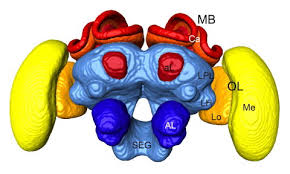
In October 2024, the FlyWire consortium published the complete connectome of an adult Drosophila melanogaster brain: 139,255 neurons, 54.5 million synapses, 8,453 cell types, mapped at 8-nanometer resolution. This is only the third complete animal connectome ever produced, following C. elegans (302 neurons, 1986) and Drosophila larva (3,016 neurons, 2023). The 38-year gap between the first and third isn’t just a story about technology—it’s about fundamental scaling constraints that apply equally to biological neural networks and autonomous robotics.

A connectome is the complete wiring diagram of a nervous system. Think of it as the ultimate circuit board schematic, except instead of copper traces and resistors, you’re mapping biological neurons and the synapses that connect them. But unlike an electrical circuit you can trace with your finger, these connections exist in three-dimensional space at scales invisible to the naked eye. A single neuron might be a tenth of a millimeter long but only a few microns wide—about 1/20th the width of a human hair. The synapses where neurons connect are even tinier: just 20-40 nanometers across, roughly 2,000 times smaller than the width of a hair. And there are millions of them, tangled together in a three-dimensional mesh that makes the densest urban skyline look spacious by comparison. The connectome doesn’t just tell you which neurons exist—it tells you how they talk to each other. Neuron A connects to neurons B, C, and D. Neuron B connects back to A and forward to E. That recurrent loop between A and B? That might be how the fly remembers the smell of rotting fruit. The connection strength between neurons—whether a synapse is strong or weak—determines whether a signal gets amplified or filtered out. It’s the difference between a whisper and a shout, between a fleeting thought and a committed decision.

Creating a connectome is almost absurdly difficult. First, you preserve the brain perfectly at nanometer resolution, then slice it into thousands of impossibly thin sections—the fruit fly required 7,000 slices, each just 40 nanometers thick, about 1/1,000th the thickness of paper, cut with diamond-knife precision. Each slice goes under an electron microscope, generating a 100-teravoxel dataset where each pixel represents an 8-nanometer cube of brain tissue. Then comes the nightmare part: tracing each neuron through all 7,000 slices, like following a single thread through 7,000 sheets of paper where the thread appears as just a dot on each sheet—and there are 139,255 threads tangled together. When Sydney Brenner’s team mapped C. elegans in the 1970s and 80s, they did this entirely by hand, printing electron microscopy images on glossy paper and tracing neurons with colored pens through thousands of images. It took 15 years for 302 neurons. The fruit fly has 460 times more.

This is where the breakthrough happened. The FlyWire consortium used machine learning algorithms called flood-filling networks to automatically segment neurons, but the AI made mistakes constantly—merging neurons, splitting single cells into pieces, missing connections. So they crowdsourced the proofreading: hundreds of scientists and citizen scientists corrected errors neuron by neuron, synapse by synapse, and the AI learned from each correction. This hybrid approach—silicon intelligence for speed, human intelligence for accuracy—took approximately 50 person-years of work. The team then used additional machine learning to predict neurotransmitter types from images alone and identified 8,453 distinct cell types. The final result: 139,255 neurons, 54.5 million synapses, every single connection mapped—a complete wiring diagram of how a fly thinks.

The O(n²) Problem

Connectomes scale brutally. Going from 302 to 139,255 neurons isn’t 460× harder—it’s exponentially harder because connectivity scales roughly as n². The worm has ~7,000 synapses. The fly has 54.5 million—a 7,800× increase in edges for a 460× increase in nodes. The fly brain also went from 118 cell classes to 8,453 distinct types, meaning the segmentation problem became orders of magnitude more complex.

Sydney Brenner’s team in 1986 traced C. elegans by hand through 8,000 electron microscopy images using colored pens on glossy prints. They tried automating it with a Modular I computer (64 KB memory), but 1980s hardware couldn’t handle the reconstruction. The entire project took 15 years.

The FlyWire consortium solved the scaling problem with a three-stage pipeline:

Exponential Growth

460× more neurons in 38 years

7,142× more synapses

Complexity: O(n²) connections

Stage 1: Automated segmentation via flood-filling networks
They sliced the fly brain into 7,000 sections at 40nm thickness (1/1000th the thickness of paper), generating a 100-teravoxel dataset. Flood-filling neural networks performed initial segmentation—essentially a 3D region-growing algorithm that propagates labels across voxels with similar appearance. This is computationally tractable because it’s local and parallelizable, but error-prone because neurons can look similar to surrounding tissue at boundaries.

Stage 2: Crowdsourced proofreading
The AI merged adjacent neurons, split single cells, and missed synapses constantly. Hundreds of neuroscientists and citizen scientists corrected these errors through a web interface. Each correction fed back into the training set, iteratively improving the model. This hybrid approach—automated first-pass, human verification, iterative refinement—consumed approximately 50 person-years.

Stage 3: Machine learning for neurotransmitter prediction
Rather than requiring chemical labeling for every neuron, they trained classifiers to predict neurotransmitter type (glutamate, GABA, acetylcholine, etc.) directly from EM morphology. This is non-trivial because neurotransmitter identity isn’t always apparent from structure alone, but statistical patterns in vesicle density, synapse morphology, and connectivity motifs provide signal.

The result is complete: every neuron traced from dendrite to axon terminal, every synapse identified and typed, every connection mapped. UC Berkeley researchers ran the entire connectome as a leaky integrate-and-fire network on a laptop, successfully predicting sensorimotor pathways for sugar sensing, water detection, and proboscis extension. Completeness matters because partial connectomes can’t capture whole-brain dynamics—recurrent loops, feedback pathways, and emergent computation require the full graph.

50 largest neurons of the fly brain connectome.
Credit: Tyler Sloan and Amy Sterling for FlyWire, Princeton University, (Dorkenwald et al., 2024)

Power Scaling: The Fundamental Constraint

Here’s the engineering problem: the fly brain operates on 5-10 microwatts. That’s 0.036-0.072 nanowatts per neuron. It enables:

Controlled flight at 5 m/s with 200 Hz wing beat frequency
Visual processing through 77,536 optic lobe neurons at ~200 fps
Real-time sensorimotor integration with ~10ms latencies
Onboard learning and memory formation
Navigation, courtship, and decision-making

Compare this to autonomous systems:

System	Power	Capability	Efficiency
Fruit fly brain	10 μW	Full autonomy	0.072 nW/neuron
Intel Loihi 2	2.26 μW/neuron	Inference only	31× worse than fly
NVIDIA Jetson (edge inference)	~15 W	Vision + control	10⁶× worse
Boston Dynamics Spot	~400 W total	90 min runtime	–
Human brain	20 W	1 exaFLOP equivalent	50 pFLOPS/W
Frontier supercomputer	20 MW	1 exaFLOP	50 FLOPS/W

The brain achieves ~10¹² better energy efficiency than conventional computing at the same computational throughput. This isn’t a transistor physics problem—it’s architectural.

Why Biology Wins: Event-Driven Sparse Computation

The connectome reveals three principles that explain biological efficiency:

1. Asynchronous event-driven processing
Neurons fire sparsely (~1-10 Hz average) and asynchronously. There’s no global clock. Computation happens only when a spike arrives. In the fly brain, within four synaptic hops nearly every neuron can influence every other (high recurrence), yet the network remains stable because most neurons are silent most of the time. Contrast this with synchronous processors where every transistor is clocked every cycle, consuming 30-40% of chip power just on clock distribution—even when idle.

2. Strong/weak connection asymmetry
The fly connectome shows that 70-79% of all synaptic weight is concentrated in just 16% of connections. These strong connections (>10 synapses between a neuron pair) carry reliable signals with high SNR. Weak connections (1-2 synapses) may represent developmental noise, context-dependent modulation, or exploratory wiring that rarely fires. This creates a core network of reliable pathways overlaid with a sparse exploratory graph—essentially a biological ensemble method that balances exploitation and exploration.

3. Recurrent loops instead of deep feedforward hierarchies
The Drosophila larval connectome (3,016 neurons, 548,000 synapses) revealed that 41% of neurons receive long-range recurrent input. Rather than the deep feedforward architectures in CNNs (which require many layers to build useful representations), insect brains use nested recurrent loops. This compensates for shallow depth: instead of composing features through 50+ layers, they iterate and refine through recurrent processing with 3-4 layers. Multisensory integration starts with sense-specific second-order neurons but rapidly converges to shared third/fourth-order processing—biological transfer learning that amortizes computation across modalities.

Neuromorphic Implementations: Narrowing the Gap

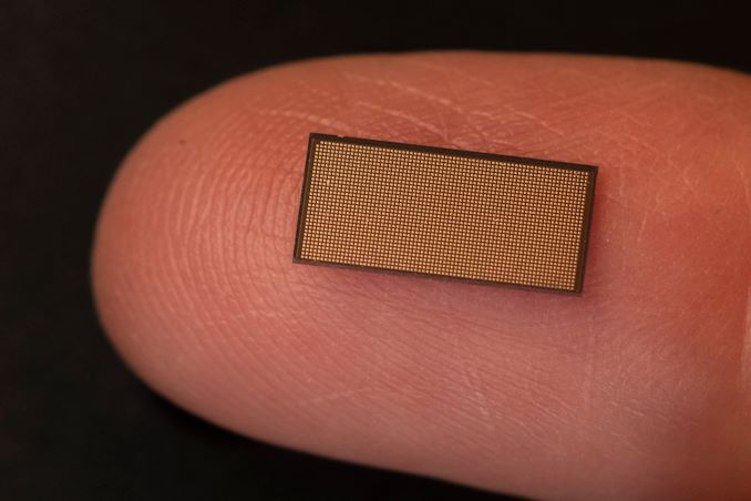
Event-driven neuromorphic chips implement these principles in silicon:

Intel Loihi 2 (2024)

1M neurons/chip, 4nm process
Fully programmable neuron models
Graded spikes (not just binary)
2.26 μW/neuron (vs. 0.072 nW for flies—still 31,000× worse)
16× better energy efficiency than GPUs on audio tasks

The Hala Point system (1,152 Loihi 2 chips) achieves 1.15 billion neurons at 2,600W maximum—demonstrating that neuromorphic scales, but still consumes orders of magnitude more than biology per neuron.

IBM NorthPole (2023)

Eliminates von Neumann bottleneck by co-locating memory and compute
22 billion transistors, 800 mm² die
25× better energy efficiency vs. 12nm GPUs on vision tasks
72× better efficiency on LLM token generation

NorthPole is significant because it addresses the memory wall: in traditional architectures, moving data between DRAM and compute costs 100-1000× more energy than the actual computation. Co-locating memory eliminates this overhead.

BrainChip Akida (2021-present)

First commercially available neuromorphic chip
100 μW to 300 mW depending on workload
Akida Pico (Oct 2024): <1 mW operation
On-chip learning without backprop

The critical insight: event-driven cameras + neuromorphic processors. Traditional cameras output full frames at 30-60 fps whether or not anything changed. Event-based cameras (DVS sensors) output asynchronous pixel-level changes only—mimicking retinal spike encoding. Paired with neuromorphic processors, this achieves dramatic efficiency: idle power drops from ~30W (GPU) to <1mW (neuromorphic).

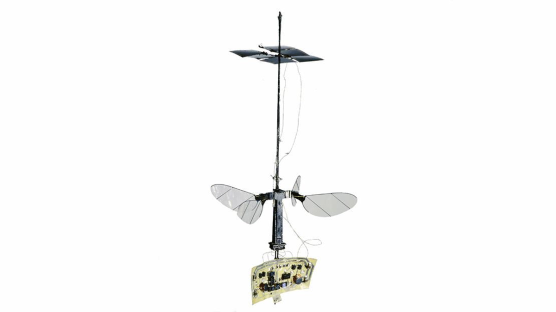
RoboBees
Credit: Wyss Institute at Harvard University

The Micro-Robotics Power Wall

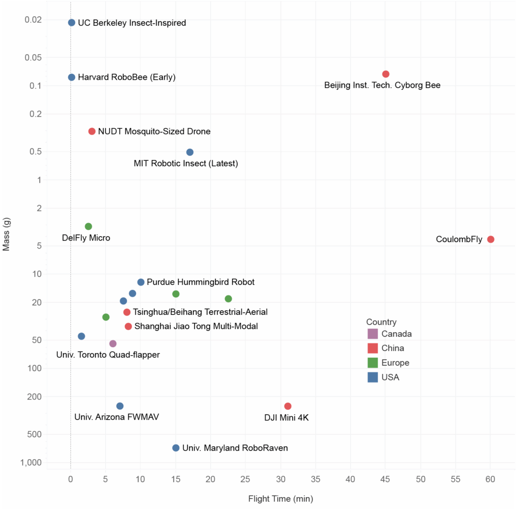
The scaling problem becomes acute at insect scale. Harvard’s RoboBee (80-100 mg, 3 cm wingspan) flies at 120 mW. Solar cells deliver 0.76 mW/mg at full sun—but the RoboBee needs 3× Earth’s solar flux to sustain flight. This forces operation under halogen lights in the lab, not outdoor autonomy.

The fundamental constraint is energy storage scaling. As robots shrink, surface area (power collection) scales as r², volume (power demand) as r³. At sub-gram scale, lithium-ion provides 1.8 MJ/kg. Metabolic fat provides 38 MJ/kg—a 21× advantage that no battery chemistry on the roadmap approaches.

This creates a catch-22: larger batteries enable longer flight, but add weight requiring bigger actuators drawing more power, requiring even larger batteries. The loop doesn’t converge.

Alternative approaches:

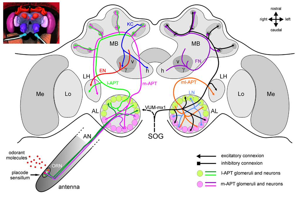
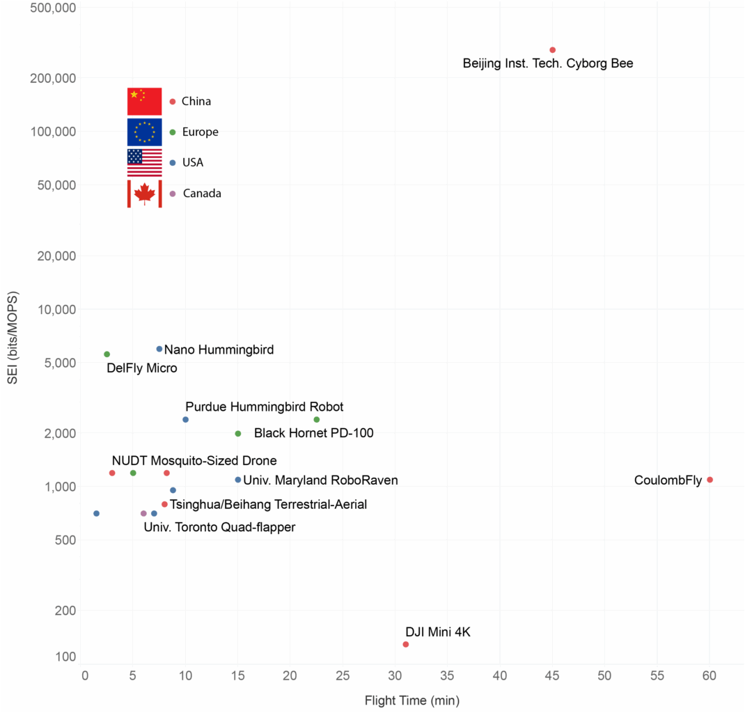
Cyborg insects: Beijing Institute of Technology’s 74 mg brain controller interfaces directly with bee neural tissue via three electrodes, achieving 90% command compliance. Power: hundreds of microwatts for control electronics. Propulsion: biological, running on metabolic fuel. Result: 1,000× power advantage over fully robotic micro-flyers.
Chemical fuels: The RoBeetle (88 mg crawling robot) uses catalytic methanol combustion. Methanol: 20 MJ/kg—10× lithium-ion density. But scaling combustion to aerial vehicles introduces complexity (fuel pumps, thermal management) at millimeter scales.
Tethered operation: MIT’s micro-robot achieved 1,000+ seconds of flight with double aerial flips, but remains tethered to external power.

For untethered autonomous micro-aerial vehicles, current battery chemistry makes hour-long operation physically impossible.

The Dragonfly Algorithm: Proof of Concept

The dragonfly demonstrates what’s possible with ~1 million neurons. It intercepts prey with 95%+ success, responding to maneuvers in 50ms:

10 ms: photoreceptor response + signal transmission
5 ms: muscle force production
35 ms: neural computation

That’s 3-4 neuron layers maximum at biological signaling speeds (~1 m/s propagation, ~1 ms synaptic delays). The algorithm is parallel navigation: maintain constant line-of-sight angle to prey while adjusting speed. It’s simple, fast, and works with 1/100th the spatial resolution of human vision at 200 fps.

The dragonfly’s visual system contains 441 input neurons feeding 194,481 processing neurons. Researchers have implemented this in III-V nanowire optoelectronics operating at sub-picowatt per neuron. The human brain averages 0.23 nW/neuron—still 100,000× more efficient than conventional processors per operation. Loihi 2 and NorthPole narrow this to ~1,000× gap, but the remaining distance requires architectural innovation, not just process shrinks.

Distributed Control vs. Centralized Bottlenecks

Insect nervous systems demonstrate distributed control:

Spinal reflexes: 10-30 ms responses without brain involvement
Central pattern generators: rhythmic movements (walking, flying) produced locally in ganglia
Parallel sensory streams: no serialization bottleneck

Modern autonomous vehicles route all sensor data to central compute clusters, creating communication bottlenecks and single points of failure. The biological approach is hierarchical:

Low-level reactive control: fast (1-10 ms), continuous, local
High-level deliberative planning: slow (100-1000 ms), occasional, centralized

This matches the insect architecture: local ganglia handle reflexes and pattern generation, brain handles navigation and decision-making. The division of labor minimizes communication overhead and reduces latency.

Scaling Constraints Across Morphologies

The power constraint manifests predictably across scales:

Micro-aerial (0.1-1 g): Battery energy density is the hard limit. Flight times measured in minutes. Solutions require chemical fuels, cyborg approaches, or accepting tethered operation.

Drones (0.1-10 kg): Power ∝ v³ for flight. Consumer drones: 20-30 min. Advanced commercial: 40-55 min. Headwinds cut range by half. Monarch butterflies migrate thousands of km on 140 mg of fat—200× better mass-adjusted efficiency.

Ground robots (10-100 kg): Legged locomotion is 2-5× less efficient than wheeled for the same distance (constantly fighting gravity during stance phase). Spot: 90 min runtime, 3-5 km range. Humanoids: 5-10× worse cost of transport than humans despite electric motors being more efficient than muscle (90% vs. 25%). The difference is energy storage and integrated control.

Computation overhead: At large scale (vehicles drawing 10-30 kW), AI processing (500-1000W) is 5-10% overhead. At micro-scale, computation dominates: a 3cm autonomous robot with CNN vision gets 15 minutes from a 40 mAh battery because video processing drains faster than actuation.

The Engineering Path Forward

The connectome provides a blueprint, but implementation requires system-level integration:

1. Neuromorphic processors for always-on sensing
Event-driven computation with DVS cameras enables <1 mW idle power. Critical for battery-limited mobile robots.

2. Hierarchical control architectures
Distribute reflexes and pattern generation to local controllers. Reserve central compute for high-level planning. Reduces communication overhead and latency.

3. Task-specific optimization over general intelligence
The dragonfly’s parallel navigation algorithm is simple, fast, and sufficient for 95%+ interception success. General-purpose autonomy is expensive. Narrow, well-defined missions allow exploiting biological efficiency principles.

4. Structural batteries and variable impedance actuators
Structural batteries serve as both energy storage and load-bearing elements, improving payload mass fraction. Variable impedance actuators mimic muscle compliance, reducing energy waste during impacts.

5. Chemical fuels for micro-robotics
At sub-gram scale, metabolic fuel’s 20-40× energy density advantage over batteries is insurmountable with current chemistry. Methanol combustion, hydrogen fuel cells, or cyborg approaches are the only paths to hour-long micro-aerial autonomy.

Minuscule RoBeetle Turns Liquid Methanol Into Muscle Power
Credit: IEEE Spectrum

Conclusion: Efficiency is the Constraint

The fruit fly connectome took 38 years after C. elegans because complexity scales exponentially. The same scaling laws govern autonomous robotics: every doubling of capability demands exponentially more energy, computation, and integration complexity.

The fly brain’s 5-10 μW budget for full autonomy isn’t just impressive—it’s the benchmark. Current neuromorphic chips are 1,000-30,000× worse per neuron. Closing this gap requires implementing biological principles: event-driven sparse computation, strong/weak connection asymmetry, recurrent processing over deep hierarchies, and distributed control.

Companies building autonomous systems without addressing energetics will hit a wall—the same wall that kept connectomics at 302 neurons for 38 years. Physics doesn’t care about better perception models if the robot runs out of power before completing useful work.

When robotics achieves even 1% of biological efficiency at scale, truly autonomous micro-robots become feasible. Until then, the scaling laws remain unforgiving. The connectome reveals both how far we are from biological efficiency—and the specific architectural principles required to close that gap.

The message for robotics engineers: efficiency isn’t a feature, it’s the product.

Explore the full FlyWire visualization at https://flywire.ai/

October 16, 2025 (updated October 17, 2025) By Tim Booher 3 Comments

Engineering & Code

The GENIUS Act: From Crypto Experiment to National Security Infrastructure

When President Trump signed the GENIUS Act on July 18, 2025, he didn’t just regulate stablecoins—he legitimized an entire technology stack that will become core infrastructure for defense and intelligence agencies. By requiring full liquid reserves and exempting compliant stablecoins from securities regulations, the Act transforms what was once speculative technology into government-grade payment and settlement infrastructure.

This matters because modern military operations aren’t starved for bandwidth and processing power—they need immutable state, enforceable trust, and precise data distribution. The same technology that powers a dollar-pegged stablecoin can lock mission events in seconds, encode rules of engagement in self-executing code, and prove compliance without compromising operational security.

Command and control breaks when everyone maintains their own version of “truth.” Byzantine fault-tolerant consensus—the same mechanism that prevents double-spending in stablecoins—forces independent nodes to agree on each state change before it’s recorded. No more reconciliation queues. No more debating which ROE update is authoritative. Just a single, cryptographically locked sequence of events that can’t be quietly rewritten.

With that single, tamper‑proof log in place, autonomous systems can graduate from lone‑wolf behaviors to coordinated swarms: the ledger’s state becomes the authoritative “leader,” while each drone, satellite, or ground robot is a “follower” that subscribes to—and writes into—the same stream. AI planners can post composite tasks (sensor → shooter chains, refuel rendezvous, med‑evac corridors) as smart‑contract directives; individual platforms claim subtasks, stake cryptographic commitments, and update status the moment they act. Because every node sees identical state within seconds, hand‑offs and deconfliction happen in code, not over voice nets, and higher‑level orchestration engines can reason over the evolving mission graph in real time. The result is multi‑platform C2 where machines negotiate roles, verify execution, and re‑task themselves under a commander’s intent—while commanders and auditors retain an immutable play‑by‑play of who led, who followed, and whether the AI kept faith with policy.

But this tech can do more than just enable coordinated higher level autonomy. Supply chains fail when we can’t prove provenance. The tokenization standards legitimized by the GENIUS Act give every part, payment, and piece of data a cryptographic birth certificate. A counterfeit component breaks the chain instantly. Payment releases automatically when secure oracles confirm delivery and compliance. Cash cycles drop from 60-120 days to near real-time.

Zero-trust architectures stall without programmable policy. Smart contracts—now legally deployable for government use—convert access control from organizational charts into mathematical proofs. A fire mission only executes if the required cryptographic signatures align. Coalition partners can verify actions without seeing raw intelligence.

Before the GENIUS Act, stable‑coin rails and tokenised provenance rarely moved beyond DARPA demos because the scale‑up money wasn’t there: mission engineers could prove value in a sandbox, but CFOs and contracting officers lacked a legally accepted funding mechanism and a clear path to classify the R&D spend. The existence of large‑volume pilots—and the capital that follows—will harden the stack, integrate it with legacy systems, and drive down technical risk for the war‑fighter.

Now, with explicit statutory protection for properly-backed digital assets, defense contractors can build at scale. The same legal framework that protects a stablecoin’s dollar peg protects a tokenized part inventory, a programmable budget line, or a cryptographically-governed sensor feed.

The Act doesn’t just permit this infrastructure—it demands it. Full reserve requirements and regular attestations? That’s exactly the level of auditability the DoD needs for financial management. Bankruptcy-remote custody structures? Perfect for protecting government assets in contractor systems. Real-time settlement with cryptographic finality? Precisely what accelerated kill chains require.

The GENIUS Act creates a rare alignment between financial innovation and national security needs. The question isn’t whether this technology will reshape defense operations—it’s who will build it.

This will intersect with formal methods in a powerful way. Recent breakthroughs in large‑scale formal verification—driven by Amazon’s Byron Cook and Michael Hicks—slot perfectly into this Merkle‑anchored world: their push‑button model‑checking and property‑based compilation pipelines can exhaustively prove that a smart contract (or autonomous‑agent policy) preserves invariants like “never fire without dual‑key authorization” or “funds only move when supply‑chain proofs are valid” before the code ever deploys, while the Merkle tree records every compiled binary and configuration hash so field auditors can show the running system is exactly the one that passed the proofs.

Silicon Valley fintechs are already racing to capture the civilian market. They’ll build the protocols, control the standards, and rent access back to the government. Or defense primes can recognize this moment: the regulatory green light to build sovereign, military-grade distributed systems that we control from the ground up.

The experimental phase is over. The GENIUS Act provides the legal foundation. The technology works at massive scale. The operational need is real.

The only question left is whether the national security establishment will seize this opportunity to build its own cryptographic infrastructure—or wake up in five years dependent on systems designed for retail banking, hoping they can be retrofitted for combat.

July 25, 2025 (updated July 25, 2025) By Tim Booher One Comment

Autonomy

Robot Bees and other Little Robots

Researchers in China are crafting cyborg bees by fitting them with incredibly thin neural implants (article: Design of flight control system for honeybee based on EEG stimulation). The story isn’t that biology replaces electronics; it’s that biology supplies free actuation, sensing, and ultra low power computation that we can piggyback on with just enough silicon to plug those abilities into our digital world. Through leveraging natural flight capabilities and endurance of biological hosts, you have an ideal covert reconnaissance or delivery platform ideal for military surveillance, counterterrorism operations, physically hacking hardware and disaster relief missions where traditional drones would be too conspicuous or lack the agility to navigate complex environments.

So, there are lots of news articles on this, but the concept of miniature flying machines is far from new. For over a decade before projects like Harvard’s pioneering RoboBee took flight in 2007, researchers were already delving into micro-aerial vehicles (MAVs), driven by the quest for stealthy surveillance and other specialized applications. Early breakthroughs, such as the untethered flight of the Delft University of Technology’s “DelFly,” laid crucial groundwork, proving that insect-scale flight was not just a sci-fi dream but an achievable engineering challenge. This long history underscores a persistent, fascinating pursuit: shrinking aerial capabilities to an almost invisible scale.

Unlike the “China has a robot Bee!” articles, I wanted to step back and survey this space and where it’s going, and, well, this is kinda a big deal. The plot below reveals the tug-of-war between a robot’s mass and its flight endurance. While a general trend shows heavier robots flying longer, the interesting data are in the extremes. Beijing’s “Cyborg Bee” is a stunning outlier, achieving incredible flight times (around 45 minutes) with a minuscule 0.074-gram control unit by cleverly outsourcing the heavy lifting to a living bee – a biological cheat code for endurance. Conversely, the “NUDT Mosquito-Sized Drone” pushes miniaturization to its absolute limit at 0.3 grams, but sacrifices practical flight time, lasting only a few minutes . This highlights the persistent “holy grail” challenge: building truly insect-scale artificial robots that can fly far–and obey orders. Even cutting-edge artificial designs like MIT’s latest robotic insect, while achieving an impressive 17 minutes of flight, still carry more mass than their biological counterparts. The plot vividly demonstrates that while human ingenuity can shrink technology to astonishing scales, nature’s efficiency in flight remains the ultimate benchmark.

Researchers figured out how to deliver precise electronic pulses that create rough sensory illusions, compelling the bee to execute flight commands—turning left or right, advancing forward, or retreating on demand. And this works. During laboratory demonstrations, these bio-hybrid drones achieved a remarkable 90% command compliance rate, following directional instructions with near-perfect accuracy. By hijacking the bee’s neural pathways, China has effectively weaponized nature’s own engineering, creating a new class of biological surveillance assets that combine the stealth of living organisms with the precision of electronic control systems.

The Beijing team’s breakthrough lies in their precise neural hijacking methodology: three hair-width platinum-iridium micro-needles penetrate the bee’s protocerebrum, delivering charge-balanced biphasic square-wave pulses at a soothing ±20 microamperes—just above the 5-10 µA activation threshold for insect CNS axons yet safely below tissue damage limits. These engineered waveforms, typically running at 200-300 Hz to mimic natural flight central pattern generators, create directional illusions rather than forcing specific muscle commands. Each pulse lasts 100-300 microseconds, optimized to match the chronaxie of 2-4 micrometer diameter insect axons.

Figuring this out is more guessing than careful math. Researchers discovered these “magic numbers” through systematic parametric sweeps across amplitude (5-50 µA), frequency (50-400 Hz), and pulse width (50-500 µs) grids, scoring binary outcomes like “turn angle >30°” until convergence on optimal control surfaces. Modern implementations use closed-loop Bayesian optimization with onboard IMUs and nRF24L01 radios, reducing tuning time from hours to ~90 seconds while adding ±10% amplitude jitter to counteract the bee’s rapid habituation response.

You can’t figure this out on live bees. To get these measurements, the honeybee head capsule is isolated from the body while leaving the entire brain undamaged. The head is cut free and placed into a dye-loaded and cooled ringer solution in a staining chamber for 1 hour, then fixed in a recording chamber, covered with a cover-slip, and imaged under the microscope. After you do this, you can conduct experiments on hundreds of honeybees using low and high current intensity. After stimulation, the Isolated Pulse Stimulator was modulated to generate a dissociating pulse (20 µA DC, 15–20 s), which partially dissociated Fe³⁺ from the stimulating electrode and deposited it in surrounding brain tissue marking where they stimulated for post-mortem analysis.

Precise probe placement relies on decades of accumulated neuroanatomical knowledge. Researchers leverage detailed brain atlases created through electron microscopy and confocal imaging, which map neural structures down to individual synaptic connections. Before inserting stimulation electrodes, they consult these three-dimensional brain maps to target specific neural clusters with sub-millimeter accuracy. During experiments, they verify their targeting using complementary recording techniques: ultra-fine borosilicate glass microelectrodes with 70-120 MΩ tip resistance penetrate individual neurons, capturing their electrical chatter at 20,000 samples per second. These recordings reveal whether the stimulation reaches its intended targets—researchers can literally watch neurons fire in real-time as voltage spikes scroll across their screens, confirming that their three platinum-iridium needles are activating the correct protocerebral circuits. This dual approach—anatomical precision guided by brain atlases combined with live electrophysiological validation—ensures the cyborg control signals reach exactly where they need to go.

What was cool here is that they found a nearly linear relationship between the stimulus burst duration and generated torque. This stimulus-torque characteristic holds for burst durations of up to 500ms. Hierarchical Bayesian modeling revealed that linearity of the stimulus-torque characteristic was generally invariant, with individually varying slopes. This allowed them to get generality through statistical models accounting for individual differences.

Learning the signals is only half the battle. The power challenge defines the system’s ultimate constraints: while a flying bee dissipates ~200 milliwatts mechanically, the cyborg controller must operate within a ~10 mW mass-equivalent budget—about what a drop of nectar weighs. Current 3-milligram micro-LiPo cells provide only ~1 milliwatt-hour, forcing engineers toward energy harvesting solutions like piezoelectric thorax patches that scavenge 20-40 microwatts from wingbeats or thermoelectric films adding single-digit microwatts from body heat. Yes, the bee is the battery.

This power scarcity drives the next evolution: rather than imposing external commands, future systems will eavesdrop on the bee’s existing neural traffic—stretch receptors encoding wingbeat amplitude, Johnston’s organs signaling airspeed, and antennal lobe spikes classifying odors with <50ms latency at just 5 µW biological power. Event-driven neuromorphic processors like Intel’s Loihi 2 can decode these spike trains at <50 microjoules per inference, potentially enabling bidirectional brain-computer interfaces where artificial intelligence augments rather than overrides the insect’s 100-million-year-evolved sensorimotor algorithms.

Challenges

Power remains the fundamental bottleneck preventing sustained cyborg control. A flying bee burns through ~200 milliwatts mechanically, but the electronic backpack must survive on a mere ~10 milliwatt mass budget—equivalent to carrying a single drop of nectar. Current micro-LiPo cells weighing 3 milligrams deliver only ~1 milliwatt-hour, barely enough for minutes of operation. Engineers have turned to the bee itself as a power source: piezoelectric patches glued to the thorax harvest 20-40 microwatts from wingbeat vibrations, while thermoelectric films capture single-digit microwatts from body heat. Combined, these provide just enough juice for duty-cycled neural recording and simple radio backscatter—but not continuous control. The thermal constraint is equally brutal: even 5 milliwatts of continuous power dissipation heats the bee’s dorsal thorax by 1°C, disrupting its olfactory navigation. This forces all onboard electronics to operate in the sub-milliwatt range, making every microjoule precious. The solution may lie in passive eavesdropping rather than active control—tapping into the bee’s existing 5-microwatt neural signals instead of imposing power-hungry external commands.

I summarize the rest of the challenges below:

Challenge	Candidate approach	Practical limits
RF antenna size	Folded‑loop 2.4 GHz BLE or sub‑GHz LoRa patterns printed on 20 µm polyimide	Needs >30 mm trace length—almost bee‑size; detunes with wing motion
Power for Tx	Ambient‑backscatter using 915 MHz carrier (reader on the ground)	100 µW budget fits; 1 kbps uplink only (ScienceDaily)
Network dynamics	Bio‑inspired swarm routing: every node rebroadcasts if SNR improves by Δ>3 dB	Scalability shown in simulation up to 5 000 nodes; real tests at NTU Singapore hit 120 roach‑bots (ScienceDaily)
Localization	Fusion of onboard IMU (20 µg) + optic‑flow + Doppler‑based ranging to readers	IMU drift acceptable for ≤30 s missions; longer tasks need visual odometry

The cyborg bee’s computational supremacy becomes stark when viewed through the lens of task efficiency rather than raw processing power. While silicon-based micro-flyers operate on ARM Cortex processors churning through 20-170 MOPS (mega-operations per second), the bee’s million-neuron brain achieves full visual navigation on just 5 MOPS—neurons firing at a leisurely 5 Hz average. This thousand-fold reduction in arithmetic operations masks a deeper truth: the bee’s sparse, event-driven neural code extracts far more navigational intelligence per computation.

$$ \text{SEI} = \frac{\text{MAP vox}/\text{sec} \times \text{Pose bits}}{\text{MOPS}}$$

To show this, I made up a metric that combines each vehicle’s vision rate, positional accuracy and onboard compute into a single “task‑efficiency” score—the Simultaneous localization and mapping (SLAM)-Efficiency Index (SEI)—so we could compare a honey‑bee brain running on microwatts with silicon drones running on megahertz. Simply put, SEI measures how many bits of world-state knowledge each platform generates per unit of processing. With SEI, the bee achieves 290,000 bits/MOPS—over 100 times better than the best silicon autopilots. Even DJI’s Mini 4K, with its 9,600 MOPS quad-core processor, manages only 420 bits/MOPS despite throwing two thousand times more compute at the problem.

This efficiency gap stems from fundamental architectural differences: bee brains process visual scenes through parallel analog channels that compress optic flow into navigation commands without digitizing every pixel, while our drones waste cycles on frame buffers and matrix multiplications. The bee’s ring-attractor neurons solve path integration as a single rotation-symmetric loop, updating its cognitive map 200 times per second (synchronized with wingbeats) using mere microwatts. Silicon systems attempting equivalent SLAM functionality—feature extraction, bundle adjustment, loop closure—burn 5-15 watts on embedded GPUs. Until neuromorphic processors can match the bee’s event-driven, power-sipping architecture, cyborg insects will remain the only sub-gram platforms capable of autonomous navigation. The chart’s below tells the story on a logarithmic scale: that lonely dot at 290,000 SEI represents not just superior engineering, but a fundamentally different computational paradigm. Note that flapping‑wing robots cluster below 200 MOPS because that’s all a 168 MHz Cortex‑M4 can supply; adding bigger processors blows the weight budget at these sizes.

The race to miniaturize autonomous flight reveals a fundamental truth about computation: raw processing power means nothing without the right architecture. While teams worldwide chase incremental improvements in battery life and chip efficiency, Beijing’s cyborg bee has leverages biology to solve this problem. Just as xAI’s Grok 4 throws trillion-parameter models at language understanding while smaller, cleaner models achieve similar results with careful data curation, bees handle similar complexity with microwatts. The lesson isn’t to abandon silicon for biology, but to recognize that sparse, event-driven architectures trump dense matrix multiplications when every microjoule counts.

Looking forward, the convergence is inevitable: neuromorphic processors like Intel’s Loihi 2 are beginning to bridge the efficiency gap, while cyborg systems like Beijing’s bee point the way toward hybrid architectures that leverage both biological and silicon strengths. The real breakthrough won’t come from making smaller batteries or faster processors—it will come from fundamentally rethinking how we encode, embed, and process information. Whether it’s Scale AI proving that better algorithms beat bigger models, or a bee’s ring-attractor neurons solving navigation with analog elegance, the message is clear: in the contest between brute force and biological intelligence, nature still holds most of the cards.

July 15, 2025 (updated July 15, 2025) By Tim Booher 5 Comments

Engineering & Code

Chinese Researchers Break 22-Bit RSA Encryption with Quantum Computer

A Chinese research team just pushed quantum computing one step closer to breaking the encryption that secures your bank account. The security that protects your credit card, banking, and private messages relies on a simple mathematical bet: it would take classical computers longer than the age of the universe to crack a 2048-bit RSA key. That bet is looking increasingly risky as quantum computers inch closer to breaking the math that secures the internet.

RSA encryption is a widely used asymmetric algorithm crucial for secure digital signatures, web browsing (SSL/TLS), online banking, messaging services, VPNs, and cloud infrastructure. The web depends on RSA and, given some recent news, it’s good to take a couple minutes and get a peek at where this is going.

This month (June 2025), researchers at Shanghai University (Wang, et al) published a study in the Chinese Journal of Computers that used a D-Wave Advantage quantum annealer to factor a 22-bit RSA integer—beating the previous 19-bit record by recasting factoring as a QUBO (Quadratic Unconstrained Binary Optimization) problem. While 22 bits falls far short of the 2048-bit keys securing the internet today, it demonstrates that quantum annealers can scale beyond past limits. The researchers demonstrated that quantum annealing can turn cryptographic attacks into combinatorial optimization problems.

Headlines can be deceptive—another Chinese group “hacked” lightweight block ciphers in 2024, and a D-Wave demo factored a contrived 2048-bit semiprime whose twin primes differed by just two bits—but genuine progress is visible in the research community.

Quantum annealers differ fundamentally from classical computers by utilizing quantum bits (qubits), which exploit phenomena like superposition and entanglement. This enables quantum annealers to efficiently solve certain optimization problems. Although limited in application compared to general-purpose quantum computers, quantum annealers’ recent progress highlights their potential impact on cryptographic security.

Quantum Annealer

Shor’s Algorithm

To make sense of this, I made a visualization to compare quantum annealing to Shor’s Algorithm. The “Quantum Annealer” side shows particles behaving in a fluid, probabilistic manner – they move chaotically and gradually converge toward a central point, representing how quantum annealers explore solution spaces by leveraging quantum superposition and tunneling effects to find optimal solutions through a process of gradual energy minimization. On the right, “Shor’s Algorithm” displays particles organizing into a rigid, structured grid pattern, illustrating the deterministic, step-by-step nature of classical quantum algorithms that follow precise mathematical procedures to solve specific problems like integer factorization. The contrast between the organic, exploratory movement on the quantum annealer side and the methodical, ordered arrangement on the classical algorithm side captures the essential difference between these two quantum computing paradigms: one uses quantum mechanics to probabilistically search for solutions, while the other uses quantum mechanics to execute deterministic algorithms with exponential speedup over classical computers.

Factoring large integers remains the yardstick for quantum progress because RSA’s safety rests on how brutally hard that task is for classical machines. Jumping from a 19-bit to a 22-bit crack looks tiny beside a 2,048-bit key, yet the pace signals that quantum methods—whether Shor’s algorithm or annealing—are gaining real traction.

RSA is safe for the moment, but the danger is time-shifted. Attackers can copy ciphertext today and decrypt it when hardware catches up, so any data that must stay private into the 2030s already needs stronger wrapping. Agencies and corporations are mapping every legacy backup, TLS endpoint, and VPN tunnel that still leans on RSA, then swapping certificates and firmware signatures for post-quantum or hybrid ones as they come up for renewal. The White House, NIST, and NSA’s CNSA 2.0 suite have turned that housekeeping into policy, naming lattice schemes such as CRYSTALS-Kyber, Dilithium, and SPHINCS+ as the new default. Migration is messy only for systems without “crypto agility,” the design principle that lets you change algorithms as easily as you update software.

Elliptic-curve keys used in Bitcoin and Ethereum sit even lower on the future quantum cost curve, but they, too, will fall once hardware scales. The immediate leak risk lies in records with decade-long value—medical histories, merger drafts, cold wallets, long-lived SSL certs—because those files are already being siphoned for eventual decryption.

Quantum road maps show why urgency is justified. Google’s 105-qubit Willow chip has crossed the error threshold for full fault tolerance, and IBM projects two thousand logical qubits by 2033—enough to threaten roughly 1,000-bit RSA keys.

Specifically, IBM’s roadmap targets a fault-tolerant quantum computer with 200 logical qubits by 2029 (Starling) and 2,000 by 2033 (Blue Jay). Under Shor’s algorithm, factoring an $n$-bit RSA key requires roughly $2n + 2$ logical qubits , so IBM’s Blue Jay could break RSA keys up to about 999 bits by 2033. Crucially, Shor also solves discrete-log problems, meaning 256-bit ECC keys—the basis for Bitcoin’s ECDSA and Ethereum’s EdDSA—would fall with far fewer qubits, making ECC instances more vulnerable to future quantum attacks than RSA at comparable classical security levels.

Start-ups betting on photonic qubits promise faster scaling, while skeptics such as Scott Aaronson note that engineering overhead grows faster than headline qubit counts suggest. Regulators aren’t waiting: Washington demands server inventories by 2027, Brussels ties NIS2 fines to quantum-safe readiness, and Beijing is pouring billions into domestic chip fabs.

Researchers track logical-qubit lifetimes, error-corrected cycles, and real factoring benchmarks rather than raw qubit totals. A lab that links thousands of physical qubits into hundreds of long-lived logical ones would mark the tipping point where costs start resembling supercomputers, not billion-dollar prototypes.

History rarely shouts as clearly as a Chinese factoring record and a government migration order in the same quarter. It’s wise to treat post-quantum upgrades as routine maintenance—rotate keys, adopt algorithm-neutral APIs, replace certificates on schedule—and a million-qubit announcement will be just another headline. Delay, and every RSA-protected archive on your network becomes a ticking clock, counting down to disclosure day.

Special thanks to Tom Berson, Brian LaMacchia and Pat Lincoln for insights into this area.

June 26, 2025 (updated June 27, 2025) By Tim Booher 0 Comments

Engineering & Code

Web visualization

Communication is the most important skill to sell your ideas. If the last decade has taught us anything, it’s that ideas don’t win because they’re right—they win because someone makes them impossible to ignore. The best communicators I’ve seen combine advanced graphics with deep understanding of a subject. I start simple and show how to get started in web graphics.

Continue reading →

June 6, 2025 (updated June 26, 2025) By Tim Booher 0 Comments

Personal Projects & Interests

Used Mountain Bike Prices

Note: Check out the app and try the model for yourself.

UPDATE: Need to incorporate Pink Bike!

Fresh off a weekend of riding in Bentonville, I realized I need to replace my 2006 Gary Fisher Cake. But I’m data driven and love figuring out a market before I dive in. I wanted more than crowd-sourced hunches about bike pricing; I wanted numbers I could trust. New mountain bikes shed value fast—roughly 30-40 % disappears in the first year, then depreciation flattens to about 8-12 % per year until the geometry or drivetrain standard goes obsolete. Carbon frames, high-end suspension, and “halo” brands (Yeti, Santa Cruz, Pivot) hold value better than entry-level aluminum builds, yet even they nosedive if a service-heavy fork or out-of-fashion wheel size is involved. Used-bike sites quote asking prices, not what bikes actually clear for, and algorithmic estimates rarely account for regional demand or component mix. So I scraped Craigslist, Facebook Marketplace, and Bicycle Blue Book, built my own price model, and now shop with a spreadsheet instead of wishful thinking—seeing at a glance whether that $2,400 Fuel EX is a bargain.

Getting the Data

To build this bike listings dataset, I used a combination of scraping tools and manual extraction strategies across three major platforms: Craigslist, Facebook Marketplace, and Bicycle Blue Book.

For Craigslist, I automated the process end-to-end. I wrote a script (download_cl_raw.py) to fetch city-specific HTML pages using a custom User-Agent and parsed embedded JSON-LD blocks to extract listing data (which you can see here). This raw data was then processed by analyze_and_load_cl.py, which parses structured fields (e.g., brand, model, year, frame material) using regexes and known brand patterns. Only well-known mountain bike brands were retained to ensure data quality.

Facebook Marketplace posed more challenges due to limited APIs and anti-bot measures. To work around this, I manually saved listing pages via the Chrome Developer Tools (see my data here), then used BeautifulSoup (facebook_parser.py) to extract the price, location, and other specs from the HTML. Brand and model parsing reused similar regex-based logic.

For Bicycle Blue Book, I also manually downloaded the listing HTML (data here) and used a script (bb_extractor.py) to extract structured rows like name, type, size, and price using CSS selectors.

Finally, all listings were normalized, cleaned (e.g., prices cast from “$2,800” strings to numeric), and inserted into a fresh PostgreSQL table (bike_listings_new) using upload_bikes.py.

This multi-pronged approach resulted in 1,861 listings with high coverage of core fields like brand, model, year, and price, though fields like frame_size and suspension remain sparsely populated. The dataset now supports robust price modeling, brand comparisons, and cross-market analysis.

The most represented brands are Specialized (300 bikes), Trek (260), and Giant (118), with most listings concentrated in recent years like 2023 and 2024. Specialized alone accounts for over 100 bikes listed in 2023, showing clear popularity and availability on the secondhand market. Model year coverage spans from 2015 to 2025, with the majority of data coming from the last five years. In terms of data completeness, core fields like title, price, brand, and year are over 95% populated, while others such as frame_size, wheel_size, and drivetrain have much sparser coverage. Notably, only 20% of entries have frame_size and less than 10% have detailed mechanical specs like brake_type or suspension. This makes broad comparisons possible on price and brand, but highlights the challenges in making deeper component-level comparisons—especially since components and condition may vary significantly even within the same model and year. Nonetheless, the dataset offers a strong foundation for analyzing used bike market trends, pricing gaps between platforms, and brand popularity over time.

Some parameters I could get 100% coverage, while there was nearly no data on tires or suspension travel. You should check out this monster query to generate this table.

column_name	populated_count	missing_count	total_rows	percentage populated
id	1861	0	1861	100
city	1861	0	1861	100
post_date	1861	0	1861	100
price	1861	0	1861	100
currency	1861	0	1861	100
title	1861	0	1861	100
brand	1861	0	1861	100
scraped_at	1861	0	1861	100
source	1861	0	1861	100
model	1854	7	1861	99.62
year	1794	67	1861	96.4
frame_material	1735	126	1861	93.23
original_model	1682	179	1861	90.38
location	1679	182	1861	90.22
frame_size	378	1483	1861	20.31
url	237	1624	1861	12.74
wheel_size	173	1688	1861	9.3
drivetrain	95	1766	1861	5.1
brake_type	47	1814	1861	2.53
suspension	12	1849	1861	0.64
tire_brand	2	1859	1861	0.11
travel	1	1860	1861	0.05

Initial Observations

My first question, was how prices compare between facebook, craiglist and bicycle bluebook. Craigslist prices are systematically lower—often by 20–50%, and sometimes by multiples—for the same year+model. eg. in 2019 Switchblade: CL $1,500 vs FB $2,000 and SB150: CL $3,300 vs FB $3,600. BicycleBluebook, when present, sits between Craigslist and Facebook, acting as a mid-market reference. This supercool sql let me compare the sites.

year	model	avg craigslist	avg facebook	avg bb	abs spread	max_min ratio
2024	Marlin 6	$2,800.00	$500.00		$2,300.00	5.6
2024	Stumpjumper	$1,026.25	$2,375.00		$1,348.75	2.31
2023	Tallboy	$1,150.00	$2,600.00		$1,450.00	2.26
2023	Stumpjumper	$1,085.00	$2,371.67		$1,286.67	2.19
2024	Fuel EX 8	$1,108.33	$2,300.00		$1,191.67	2.08
2024	141	$3,500.00	$1,900.00		$1,600.00	1.84
2021	SB95	$1,500.00	$2,500.00		$1,000.00	1.67
2021	SB150	$2,000.00	$3,200.00		$1,200.00	1.6
2022	Trance X 3	$1,200.00	$1,900.00		$700.00	1.58
2023	Fuel EX 5	$856.25		$1,350.00	$493.75	1.58
2022	Spark 960	$1,849.00		$1,200.00	$649.00	1.54

When comparing average bike prices across Craigslist, Facebook, and BicycleBluebook for the same year and model, there are striking disparities. Similar spreads are evident for popular models like the Stumpjumper and Tallboy, where Facebook listings consistently command significantly higher prices. In other cases, such as the Fuel EX 8 and SB150, the Craigslist price is notably lower by over $1,000 on average. While these differences are compelling, it’s important to note that they may reflect variations in bike condition, component specs, and seller expectations rather than pure market inefficiency. Still, the consistent patterns suggest that Craigslist may offer lower-priced listings on average, while Facebook often reflects a more premium price tier.

Does the city matter?

(no, cuz this market is crazy)

From some quick analysis, most brand-model-year combinations appear in only one city, so their local average simply is the national average (100 % rows). There is just not enough clean data to answer this question and the one conclusion I take away is that bike pricing is a super inefficient market. Where a combo shows up in two markets the price gaps are striking: a 2025 “unknown” Specialized lists for $750 on Seattle’s boards— about 50 % above the national mean—while the same mystery build averages only $240 in Chicago (≈ 50 % below). Likewise, 2023 Trek “unknowns” fetch $1,348 in Denver (151 % of national) but just $433 in Los Angeles (49 %). Even with tiny sample sizes (3–5 bikes each), the pattern suggests regional demand and seller optimism can swing asking prices for identical vintage-and-brand bikes by a factor of two or more.

A more sophisticated check backs this up. Only one usable “city” dummy survived the frequency filter, and LightGBM never bothered to split on it—its total gain and split count are both zero. When we rebuilt the model with the city column entirely removed, the median-absolute-error stayed exactly the same ($1,082). In short, regional location adds no predictive power in this data; age, brand, and frame material explain nearly all of the price variation we can capture, while the city a bike is listed in appears irrelevant.

Model

I built a model to sift through thousands of real listings—accounting for brand reputation, frame material, the bike’s age, and even how prices vary from city to city—to predict a fair, middle-of-the-road price in seconds. Think of it as my own personal Kelley Blue Book for bikes.

Under the hood, the valuation engine marries a classic machine-learning preprocessing stack with a modern gradient-boosted quantile regressor. Continuous bike attributes (age, log-age) sail through a median-imputer, while brand, frame material, size, and city are one-hot–encoded with frequency pruning so the feature matrix stays lean even as new makes appear. I trained with GroupKFold keyed on city—crucial for second-hand markets where geography drives pricing—to guarantee our test fold is a truly out-of-town set. A ridge model gives a transparent linear baseline, but the production scorer is a LightGBM quantile model at $\alpha = 0.5$, which directly learns the market median. Boosting captures the steep price cliffs between prestige brands and commodity frames, while quantile loss hedges against outliers that plague classifieds. The result is a file-light pipeline (preprocessor + model serialized at ~ MBs) that returns instant, geographically realistic price medians—ideal for auto-pricing listings, negotiating buys, or flagging bargains the moment they’re scraped.

You can see all the code and results here at my google colab.

Top features by total gain:
                         feature      score
4   cat__frame_material_Aluminum  83.397947
0                       num__age  40.415536
3  cat__brand_infrequent_sklearn  29.515867
5     cat__frame_material_Carbon  15.131043
1                   num__log_age   8.443574
2          cat__brand_Santa Cruz   5.624613
6        cat__frame_size_missing   0.000000
7           cat__city_Fort Worth   0.000000

The LightGBM model’s own score-gain metrics say the single most powerful signal in predicting a used-bike’s median price is simply whether the frame is aluminum (gain ≈ 83). In other words, the algorithm most often chooses to split first on “Aluminum vs. everything else,” because that decision alone lops the most error off its price guesses. Classic depreciation comes next: the bike’s age in years carries roughly half as much influence (gain ≈ 40), confirming that time on the trail is the second-biggest driver of resale value. A close third is an umbrella flag for infrequent or boutique brands—if a listing’s brand falls outside the mainstream, the model adjusts sharply (gain ≈ 30). Carbon frames still matter but noticeably less than aluminum/other (gain ≈ 15), and finally the log-age term (gain ≈ 8) offers the model a gentle curve to fine-tune how price drops level off as bikes get very old. Funny to see the Santa Cruz brand effect too.

Net takeaway: material and time dominate; brand prestige matters mainly at the extremes, and once the model knows those things, everything else is icing.

May 27, 2025 (updated June 15, 2025) By Tim Booher One Comment

The Biblical Framework or What Christian Scripture Actually Says

Revelation’s Vision: Israel in God’s Future

The Talmud Question: Corruption vs. Apostasy

Luther’s Warning: When Evangelical Frustration Becomes Genocidal Blueprint

RESEARCH REFERENCES

Tech Details

The O(n²) Problem

Connectome Evolution

Power Scaling: The Fundamental Constraint

Why Biology Wins: Event-Driven Sparse Computation

Neuromorphic Implementations: Narrowing the Gap

The Micro-Robotics Power Wall

The Dragonfly Algorithm: Proof of Concept

Distributed Control vs. Centralized Bottlenecks

Scaling Constraints Across Morphologies

The Engineering Path Forward

Conclusion: Efficiency is the Constraint

Challenges

Getting the Data

Initial Observations

Does the city matter?

Model