A very cool new compiler trick may point to a much bigger idea: a new way to think about how programs and learning fit together. In fact, this may actually be a new way to think about computation itself. The core idea is that programs can be both specified and trained.

How? Cheng Lou released a project called Handwired that takes ordinary JavaScript (conditionals, loops, state) and transforms it into the kinds of mathematical operations we associate with neural networks. This turns a program you explicitly write into something that can potentially be improved using the same learning machinery behind modern AI. That means software no longer has to be only written or only learned, it can start as a precise program and then become trainable.

You could get code started and let the real world finish it for you, picking and choosing what bits stay fixed and what parts get better.

Ok, this probably makes no sense. Let’s break it down. We have traditionally had two ways to tell computers what we want: you tell the machine what to do step by step (programming), or you show it examples and let it learn the behavior for itself (machine learning). Let’s explore these to show exactly what is new here.

For most of computing history, if you wanted a computer to do something, you wrote a program. You wrote:

if this happens:
    do this
else:
    do that

The great virtue of software is precision. A compiler takes your intent and progressively lowers it into another representation while trying very hard to preserve its semantics.

Machine learning approaches the problem from almost the opposite direction. Instead of specifying the mechanism and getting the behavior, we specify the behavior we want (through data, examples, and an objective) and let optimization discover the mechanism. With a neural network, we generally don’t know the program. We define an architecture, provide examples or an objective, initialize a huge set of parameters, calculate an error, and use gradient descent to modify those parameters until useful behavior emerges.

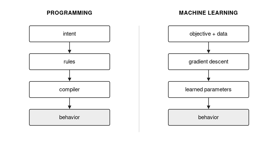
Programming gives us control. Machine learning gives us adaptability. What if we could have both?

Handwired starts with a program, not a training set or model that learns an approximation of the behavior. Take:

if a > 4:
    return 10
else:
    return 12

Handwired can transform this kind of control flow into arithmetic constructed from ReLU¹ operations and weighted values. Those operations can then be collected into the matrix-oriented representation used by neural networks.

So we get something like:

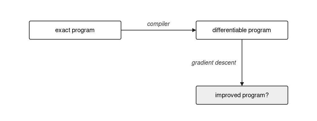
The question mark is important. We can’t assume that gradient descent magically improves any software, but the question can fundamentally change: Can I compile the program I already know into a representation that learning can subsequently modify?

I can’t tell if this has more potential to change programming or machine learning. Modern neural networks generally begin ignorant and get smarter with better data. But imagine reversing that. Suppose we start with a system that already contains substantial amounts of human knowledge: physical laws, constraints, safety rules, existing software, engineering tools, etc.

Those things don’t have to be rediscovered through training, they can be compiled in. We can then make only the places where uncertainty or optimization actually exists learnable.

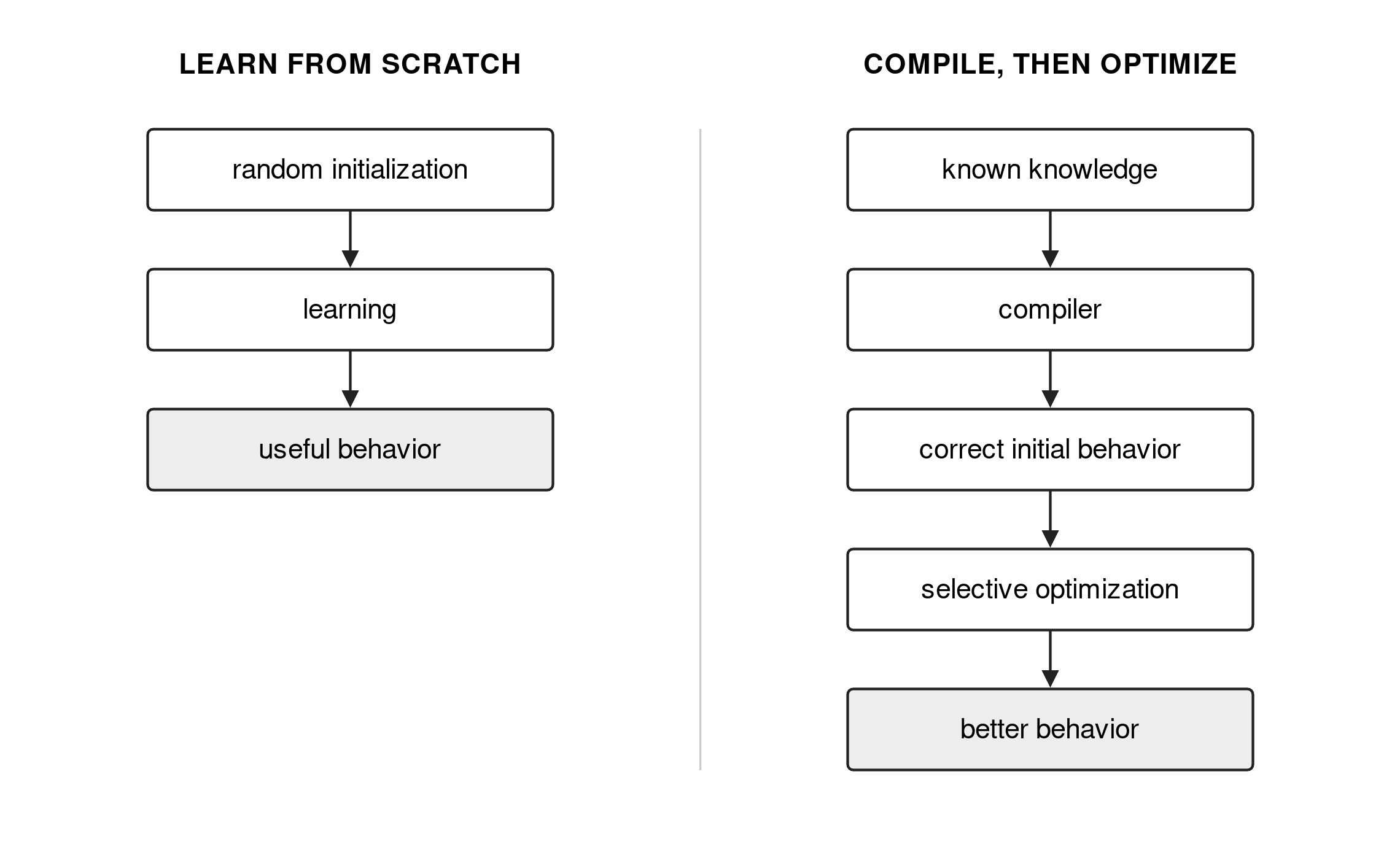
Instead of data driving the system performance, you can encode what you know about the world.

Learning becomes a refinement mechanism instead of the mechanism by which the entire system comes into existence.

This might eventually give us a very different way to build software. Imagine writing systems in which the compiler understands that different portions have different semantics with different options.

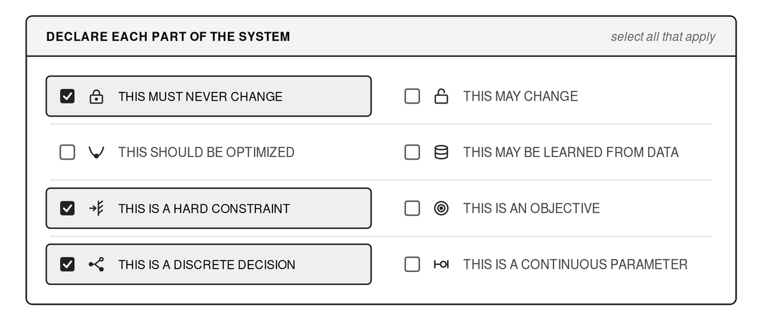
Now the compiler isn’t merely generating executable code. It is generating an optimization space. Some of the resulting representation is frozen. Some of it is trainable. Some is governed by constraints.

The boundary between “program” and “model” becomes much less rigid.

I thought about how to make this more clear interactively. Suppose we want a function that turns 0 into 1, 1 into 3, and 2 into 5, continuing the same pattern. Choose an input above and watch it travel through the box. The answer is already specified; the question mark is there because we haven’t said how the machine will produce it.

Change different input values below to set the stage for how this more complicated idea works.

This distinction is the starting point. A task describes the behavior we want: for a given input, what should the output be? The example above doesn’t yet tell us how to build that behavior. Most of us would go into SAT math problem mode and see that there is a linear equation that you can pull out of this and we would do the algebra and get:

But what if we just fed a bunch of examples to a machine learning system? It’s just another way to get a functional system. To get some intuition for this, let’s extend this basic example. Click “learn” below to see a cartoon of how a system arrives at the same capability through these two different ideas.

That is pretty basic description of the difference between a program and a machine learning model, but it sets the stage to get what is going on with Handwired.

Here we take a working program and give it a few adjustable knobs. Handwired does this by translating the program’s rules into the arithmetic of a neural network, with weights chosen to reproduce its behavior from the start.

To get this, consider a trivial program. If the input is greater than 4, return 10; otherwise, return 12. Compilation preserves those answers. But! What if we wanted to adjust this? We could re-compile a new one, or we can “unlock” one weight and introduce examples asking for 8 instead of 10.

Watch the blue dots move toward their targets as learning adjusts that answer, while the decision and the other answer stay fixed. The program supplies the starting knowledge; learning refines the part we allow to change.

Try different input values and then click “compile” below, followed by “learn” to watch the system adapt.

So with some understanding of this. What could this actually do?

First, this capability could give us a very different way to make ordinary code run faster. Handwired takes control flow that looks sequential, loops, conditionals, state, and lowers it into a small vocabulary of fast math operations. GPUs and modern ML infrastructure are extraordinarily good at executing and optimizing exactly those kinds of operations. Cheng Lou's JSON-search demo, for example, takes traditionally written JavaScript and runs the resulting computation over 100,000 documents on WebGPU in milliseconds. He also points out that once the program has been reduced to these primitives, techniques such as fusion, sparsity, and reordering become available to the compiler. This does not mean arbitrary JavaScript suddenly becomes faster on a GPU, but it raises an intriguing possibility: can we write code in a familiar sequential way and let the compiler discover a massively parallel way to execute it.

Second, a differentiable program gives us a new way to ask questions and gain deeper understanding about what the program is doing. Traditional debugging can tell us how a value flowed through a program; differentiation can potentially tell us how sensitive the final result is to values and parameters throughout that computation. In other words, instead of merely asking, “Why did I get this output?” we can sometimes ask, “Which things would most change this output, and in which direction?” This is already the basic power of automatic differentiation systems such as JAX: grad transforms a function into another function that calculates its gradient, while reverse-mode differentiation propagates information backward through a computation. Handwired's contribution is interesting because it tries to bring ordinary program structures into that same differentiable world. This isn't human-like understanding of code, but it could give software something extremely useful: a map of its own sensitivities.

Third, once you have those gradients, parts of the program can potentially optimize themselves. This is where the idea moves beyond an unusual execution strategy. Handwired's weights are initially produced by the compiler rather than learned, so the network begins by implementing the program that was written. But Cheng explicitly proposes unfreezing those compiler-created weights and training them. One of the project's demos already does this: its “Learned Gallery” compiles a photo-layout program, exposes adjustable weights, defines a loss based on the desired layout, and updates those weights live until the result better matches what the user drew. The important conceptual shift is that optimization does not have to start from random parameters and somehow rediscover the program. It can start from the program we already know and improve from there.

Fourth, this makes it possible for software to adapt differently to different people. Imagine that the fundamental rules of an application remain frozen, but particular parameters (layout, thresholds, ranking behavior, defaults, perhaps even pieces of a workflow) are allowed to adapt against an objective derived from how an individual uses it. Handwired does not yet demonstrate a general-purpose self-personalizing application, so this part is a direction rather than a result. But the mechanism is visible: the Learned Gallery changes its parameters in response to a user's desired layout, and Cheng explicitly suggests attaching a specific frozen program to a generic neural network and training the combined system end-to-end. That suggests an interesting alternative to today's personalization systems: instead of putting an AI model beside the application, parts of the application itself could become trainable while the rest remains fixed.

Finally, the biggest implication may be a new way of deciding what software actually is. We have traditionally separated programs, where humans specify behavior, from machine-learning models, where optimization discovers behavior. Handwired suggests a middle ground. A future program might contain things that are immutable, things that are differentiable, things that can be optimized, and things that can be learned from data, all inside the same computational object. Other systems such as JAX already show how compilation, vectorization, and differentiation can be composed as transformations of programs; Handwired makes the provocative move of starting with familiar imperative program structures and compiling them into that world. The result points toward software where we can specify what we know, preserve what must remain true, and optimize what we are willing to change.

These are really incredible days to be a builder. I hope this helped make some recent research accessible.

1. A ReLU is just a very simple mathematical function:
   \( \text{ReLU}(x)=\max(0,x) \) ReLUs are useful because they are extremely simple, fast, and add the nonlinearity neural networks need to learn complex patterns. They also preserve useful gradients for positive inputs, which makes deep networks much easier to train. ↩︎