Posts tagged:

Formal Methods

Let’s get Lean

(warning: I’m not trying here to explain something to folks outside computer science, but more summarize something awesome I’m learning that is changing how I write code)

As software systems grow increasingly complex and automated, ensuring correctness becomes a monumental challenge. In a future of automatically generated code, certainty is both elusive and critical. Enter Lean, a modern interactive theorem prover designed to help you reason rigorously about your code, verify its correctness, and even prove mathematical theorems. A long term research thread of mine is to make these tools increasingly useful with the goal of building stuff faster while dramatically increasing security.

Lean is a functional programming language and interactive theorem prover created by Leonardo de Moura at Microsoft Research in 2013, now an open-source project hosted on GitHub. It facilitates writing correct and maintainable code by focusing on types and functions, enabling users to concentrate on problem-solving rather than implementation details. Lean boasts features such as type inference, first-class functions, dependent types, pattern matching, extensible syntax, hygienic macros, type classes, metaprogramming, and multithreading. It also allows verification by proving properties about functions within the language itself. Lean 4 is the latest version, supported by the active Lean community and the extensive mathematical library Mathlib. Additionally, the Lean FRO nonprofit was founded in 2023 to enhance Lean’s scalability, usability, and proof automation capabilities.

Lean is a formal proof assistant—a tool that allows you to write mathematical proofs or verify software formally. It merges powerful logical foundations with ease of use, making formal verification more approachable than ever before. It’s fully integrated with visual studio.

This matters because formal verification with Lean significantly improves software reliability, reducing bugs and enhancing safety in critical sectors such as aerospace, finance, and healthcare. Lean’s rigorous approach provides exceptional precision, enabling detection of subtle errors that traditional testing often overlooks. Additionally, Lean offers profound mathematical insights, empowering mathematicians to formally confirm intricate proofs common in advanced mathematics. If fully understanding the logic of advanced math isn’t the most powerful application of AI, I don’t know what is.

Real Example

What does the most simple lean program look like?

.
├── Hello
│   └── Basic.lean
├── Hello.lean
├── Main.lean
├── README.md
├── lake-manifest.json
├── lakefile.toml
└── lean-toolchain


In Hello/Basic.lean, we define a basic greeting:

def hello := "world"


The Hello.lean file serves as the root module, importing Hello.Basic:

import Hello.Basic

The Main.lean file combines these elements and includes a formal proof:
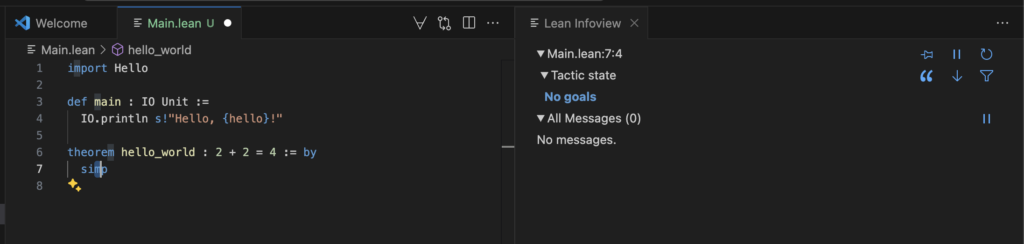
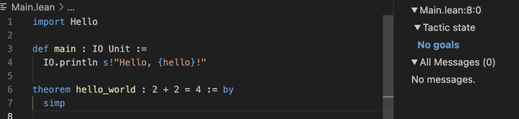
import Hello

def main : IO Unit :=
  IO.println s!"Hello, {hello}!"

theorem hello_world : 2 + 2 = 4 := by
  simp

Here, the main function prints a greeting, while the hello_world theorem demonstrates Lean’s capability to formally verify that 2 + 2 equals 4 using the simp tactic.

In Lean 4, the simp tactic is a powerful tool used to simplify goals and hypotheses by applying a collection of simplification lemmas, known as simp lemmas. These lemmas are tagged with the @[simp] attribute and are designed to rewrite expressions into simpler or more canonical forms. When invoked, simp traverses the goal or hypothesis, applying applicable simp lemmas to transform the expression step by step. For example, in proving the theorem 2 + 2 = 4, the simp tactic automatically simplifies the left-hand side to match the right-hand side, effectively completing the proof without manual intervention. This automation makes simp an essential tactic for streamlining proofs and reducing boilerplate in formal verification.

“No goals” mean the proof completes

By running lake build, Lean compiles the project and verifies the theorem. If the theorem is incorrect or the proof is invalid, Lean will provide an error, ensuring that only mathematically sound code is accepted.

This approach to software development, where code correctness is mathematically guaranteed, is especially valuable in critical systems where reliability is non-negotiable. Lean 4 empowers developers to write code that is not only functional but also formally verified, bridging the gap between programming and mathematical proof.

At this point, you are probably wondering, what Lean can really do. Every human knows 2 + 2 = 4. So let’s do something real with a real proof by induction.

-- a more interesting proof: ∀ a b, a + b = b + a
theorem add_comm (a b : Nat) : a + b = b + a := by
  induction a with
  | zero =>
    -- 0 + b = b + 0 reduces to b = b
    simp
  | succ a ih =>
    -- (a+1) + b = (b + a) + 1 by IH, then simp finishes
    simp [ih]

In this example, Lean isn’t merely checking a single arithmetic equation; it’s proving that addition on the natural numbers is commutative in full generality. By invoking the induction tactic on \(a\), Lean first establishes the base case where \(a = 0\)—showing \( + b = b + 0\) reduces to the trivial identity \(b = b\)—and then handles the inductive step, assuming \(a + b = b + a\) to prove \((a + 1) + b = b + (a + 1)\). In each case, the simp tactic automatically applies the appropriate lemmas about Nat addition to simplify both sides of the equation to the same form. Finally, when you run lake build, Lean silently compiles your code and verifies both the simple fact \(2 + 2 = 4\) and the full commutativity theorem; if any part of the proof were flawed, the build would fail, ensuring that only completely correct mathematics makes it into your code.

You can continue this to prove other properties of math.

import Hello

def main : IO Unit := do
  IO.println s!"Hello, {hello}!"
  IO.println "All proofs have been verified by Lean!"

-- trivial fact: definitionally true
theorem hello_world : 2 + 2 = 4 := by
  rfl

-- use core lemmas directly
theorem add_comm (a b : Nat) : a + b = b + a := by
  exact Nat.add_comm a b

theorem mul_add (a b c : Nat) : a * (b + c) = a * b + a * c := by
  exact Nat.mul_add a b c

For the more substantial theorems, we use the exact tactic to invoke core library lemmas directly: Nat.add_comm proves commutativity of addition \((a + b = b + a)\), and Nat.mul_add proves distributivity of multiplication over addition \((a * (b + c) = a * b + a * c)\). By relying on these already‑proven lemmas, Lean’s compiler verifies each theorem at build time—any failure in these proofs will cause lake build to error out.

Ok, so proving the basic properties of math is super cool, but how exactly is this useful? Below is an example of a “real‑world” optimization—rewriting a naive, non‑tail‑recursive summation over a list into a tail‑recursive loop—and formally verifying that the optimized version is equivalent to the original. This kind of proof is exactly what you’d need to trust that your performance tweaks haven’t changed the meaning of your code.

In embedded systems, optimization matters. The code below demonstrates how Lean can formally verify that a tail-recursive optimization is functionally equivalent to its naive counterpart—a task that’s often error-prone when done manually in traditional languages like C. The function sum is a simple, natural recursive definition that adds up all the elements of a list. It’s clear and expressive but not stack-safe for large inputs due to its non-tail-recursive form. To improve performance, we define sumAcc, which uses an explicit accumulator and a tail-recursive helper function to avoid deep call stacks. The theorem sum_correct proves that for any list of natural numbers, sum xs = sumAcc xs. This is mathematically interesting because it confirms—using structural induction and algebraic reasoning—that the transformation preserves meaning across all inputs, not just for a few test cases. In systems programming terms, this is like formally proving that a loop unrolling or inlining optimization didn’t introduce a subtle bug—a capability that’s increasingly essential as code becomes more complex and performance-critical.

import Hello
import Std.Data.List.Basic

open Std

def main : IO Unit := do
  IO.println s!"Hello, {hello}!"
  IO.println "All proofs have been verified by Lean!"

-- naive, non‑tail‑recursive sum
def sum : List Nat → Nat
| []      => 0
| x :: xs => x + sum xs

-- optimized, tail‑recursive sum using an accumulator
def sumAcc (xs : List Nat) : Nat :=
  let rec go (ys : List Nat) (acc : Nat) : Nat :=
    match ys with
    | []      => acc
    | y :: ys => go ys (acc + y)
  go xs 0

-- proof that the optimized version agrees with the naive one
theorem sum_correct (xs : List Nat) : sum xs = sumAcc xs := by
  induction xs with
  | nil =>
    -- sum [] = 0, sumAcc [] = go [] 0 = 0
    rfl
  | cons x xs ih =>
    -- sum (x :: xs) = x + sum xs
    -- sumAcc (x :: xs) = go (x :: xs) 0 = go xs (0 + x)
    -- we simplify and then apply the inductive hypothesis
    simp [sum, sumAcc]
    -- now we have: x + sum xs = sumAcc xs + x
    -- but sumAcc xs = sum xs by ih, and addition is commutative
    rw [ih]


If we were to sit down and do the math of this, it’s not straightforward:

We define two functions to compute the sum of a list of natural numbers. The first is a simple recursive version:

$$ \text{sum}([]) = 0 $$ $$ \text{sum}(x :: xs) = x + \text{sum}(xs) $$

The second is an optimized version using a tail-recursive helper function with an accumulator:

$$ \text{go}([], acc) = acc $$ $$ \text{go}(y :: ys, acc) = \text{go}(ys, acc + y) $$ $$ \text{sumAcc}(xs) = \text{go}(xs, 0) $$

We want to prove that both definitions produce the same result for any list of natural numbers:

$$ \forall xs : \text{List}(\mathbb{N}),\ \text{sum}(xs) = \text{sumAcc}(xs) $$

This is proven by structural induction on the list xs.

Base case:

$$ \text{sum}([]) = 0 $$ $$ \text{sumAcc}([]) = \text{go}([], 0) = 0 $$

Inductive step: Assume the inductive hypothesis:

$$ \text{sum}(xs) = \text{sumAcc}(xs) $$

We want to prove it holds for x :: xs:

$$ \text{sum}(x :: xs) = x + \text{sum}(xs) $$ $$ \text{sumAcc}(x :: xs) = \text{go}(x :: xs, 0) = \text{go}(xs, x) $$

By the inductive hypothesis:

$$ \text{sum}(xs) = \text{sumAcc}(xs) $$

So we substitute:

$$ x + \text{sum}(xs) = x + \text{sumAcc}(xs) $$

And from the definition of go, we know:

$$ \text{go}(xs, x) = x + \text{sumAcc}(xs) $$

Thus:

$$ \text{sum}(x :: xs) = \text{sumAcc}(x :: xs) $$

Therefore, by induction, the optimized version sumAcc is provably equivalent to the original sum for all input lists:

$$ \forall xs,\ \text{sum}(xs) = \text{sumAcc}(xs) $$

This proof ensures that the tail-recursive version retains the exact semantics of the original function—guaranteeing correctness even after performance optimization. It’s a clear example of how Lean can verify low-level loop transformations that might otherwise introduce subtle bugs in traditional systems code.

So all this hurts my head. I’m glad that software is going to do this kinda thing, and a bit in awe of the brilliance of folks who build these tools.

As software complexity grows, formal verification tools like Lean are not merely nice to have—they become essential. Companies and research institutions increasingly adopt Lean to ensure high-quality, reliable code, making Lean skills highly valuable.

Conclusion

Lean isn’t just another programming tool; it’s a powerful ally in your pursuit of correctness and reliability in mathematics and software development. Whether you’re proving intricate mathematical theorems or ensuring your software meets precise specifications, Lean is a valuable skill that promises to shape the future of reliable software and mathematics. And yes, this all complicated, but it’s super powerful, and these are exactly the powers needed as we go into a world with vibe coding, power tools and fully automated build environments. Watch this space.

By One Comment

Satisfiability modulo theories and their relevance to cyber-security

Cybersecurity and cryptoanalysis is a field filled with logic puzzles, math and numerical techniques. One of the most interesting technical areas I’ve worked goes by the name of satisfiability modulo theories (SMT) and their associated solvers. This post provides a layman’s introduction to SMT and its applications to computer science and the modern practice of learning how to break code hack.

Some background theory

Satisfiability modulo theories are a type of constraint-satisfaction problems that arise many places from software and hardware verification, to static program analysis and graph problems. They apply where logical formulas can describe a system’s states and their associated transformations. If you look under the hood for most tools used today for computer security, you will find they are based on mathematical logic as the calculus of computation. The most common constraint-satisfaction problem is propositional satisfiability (commonly called SAT) which aims to decide whether a formula composed of Boolean variables, formed using logical connectives, can be made true by choosing true/false values for its variables. In this sense, those familiar with Integer Programming will find a lot of similarities with SAT. SAT has been widely used in verification, artificial intelligence and many other areas.

As powerful as SAT problems are, what if instead of boolean constraints, we use arithmetic in a more general application to build our constraints? Often constraints are best described as linear relationships among integer or real variables. In order to understand and rigorously treat the sets involved domain theory is combined with propositional satisfiability to arrive at satisfiability modulo theory (SMT).

The satisfiability modulo theories problem is a decision problem for logical formulas with respect to combinations of background theories expressed in classical first-order logic with equality. An SMT solver decides the satisfiability of propositionally complex formulas in theories such as arithmetic and uninterpreted functions with equality. SMT solving has numerous applications in automated theorem proving, in hardware and software verification, and in scheduling and planning problems. SMT can be thought of as a form of the constraint satisfaction problem and thus a certain formalized approach to constraint programming.

The solvers developed under SMT have proven very useful in situations where linear constraints and other types of constraints are required with artificial intelligence and verification often presented as exemplars. An SMT solver can solve a SAT problem, but not vice-versa. SMT solvers draw on some of the most fundamental areas of computer science, as well as a century of symbolic logic. They combine the problem of Boolean satisfiability with domains (such as those studied in convex optimization and term-manipulating symbolic systems). Implementing SAT solvers requires an implementation of the decision problem, completeness and incompleteness of logical theories, and complexity theory.

The process of SMT solving is a procedure of finding an satisfying assignment for a quantifier-free formula for $F$ with predicates on a certain background theory $T$. Alternatively the SMT solving process could show such an assignment doesn’t exist. An assignment on all variables that satisfies these constraints is the model or $M$. $M$ will be satisified when $F$ evaluates to $\text{true}$ under a given background theory $T$. In this sense, $M$ entails $F$ under theory $T$ which is commonly expressed as: $ M \vDash_T F$. If theory $T$ is not decidable, then the underlying SMT problem is undecidable and no solver could exist. This means that given a conjunction of constraints in $T$, there must exist a procedure of finite steps that can test the existence of a satisfying assignment for these constraints.

Ok, that is a lot of jargon. What is this good for?

SMT solvers have been used since the 1970s, albeit in very specific contexts, most commonly theorem-proving cf ACL2 for some examples. More recently, SMT solvers have been helpful in test-case generation, model-based testing and static program analysis. In order to make this more real with a concrete example, let’s consider one of the most well-known operations research problems: job-shop scheduling.

If there are $n$ jobs to complete, each composed of $m$ tasks with different durations on $m$ machines. The start of a new task can be delayed indefinitely, but you can’t stop a task once it has started. For this problem, there are two constraints: precedence and resource constraints. Precedence specifies that one job has to happen before another and the resource constraint specifies that no two different tasks requiring the same machine are able to execute at the same time. If you are given a total maximum time $max$ and the duration of each task, the task is to decide if a schedule exists where the end time of every task is less than or equal to $max$ units of time. The duration of the $j$th task of job $i$ is $d_{i,j}$ and each task starts at $t_{i,j}$.

I’ve solved this problem before with heuristics such as Simulated_annealing, but you can encode the solution to this problem in SMT using the theory of linear arithmetic. First, you have to encode the precedence constraint:

$$ t_{i,j}+1 \geq t_{i,j} + d_{i,j} $$

This states that the start-time of task $j+1$ must be greater or equal to the start time of task $j$ plus its duration. The resource constraint ensures that jobs don’t overlap. Between job $i$ and job $i’$ this constraint says:

$$ (t_{i,j} \geq t_{i’,j}+d_{i’,j}) \vee (t_{i’,j} \geq t_{i,j} + d_{i,j}) $$

Lastly, each time must be non-negative, or $ t_{i,1} \geq 0 $ and the end time of the last task must be less than or equal to $max$ or $t_{i,m} + d_{i,m} \leq max$. Together, these constraints forms a logical formula that combines logical connectives (conjunctions, disjunction and negation) with atomic formulas in the form of linear arithmetic inequalities. This is the SMT formula and the solution is a mapping from the variables $t_{i,j}$ to values that make this formula $\text{true}$.

So how is this relevant to software security?

Since software uses logical formulas to describe program states and transformations between them, SMT has proven very useful to analyze, verify or test programs. In theory, if we tried every possible input to a computer program, and we could observe and understand every resultant behavior, we would know with certainty all possible vulnerabilities in a software program. The challenge of using formal methods to verify (exploit) software is to accomplish this certainty in a reasonable amount of time and this generally distills down to clever ways to reduce the state space.

For example, consider dynamic symbolic execution. In computational mathematics, algebraic or symbolic computation is a scientific area that refers to the study and development of algorithms and software for manipulating mathematical expressions and other mathematical objects. This is in contrast to scientific computing which is usually based on numerical computation with approximate floating point numbers, while symbolic computation emphasizes exact computation with expressions containing variables that are manipulated as symbols.

The software that performs symbolic calculations is called a computer algebra system. At the beginning of computer algebra, circa 1970, when common algorithms were translated into computer code, they turned out to be highly inefficient. This motivated the application of classical algebra in order to make it effective and to discover efficient algorithms. For example, Euclid’s algorithm had been known for centuries to compute polynomial greatest common divisors, but directly coding this algorithm turned out to be inefficient for polynomials over infinite fields.

Computer algebra is widely used to design the formulas that are used in numerical programs. It is also used for complete scientific computations, when purely numerical methods fail, like in public key cryptography or for some classes of non-linear problems.

To understand some of the challenges of symbolic computation, consider basic associative operations like addition and multiplication. The standard way to deal with associativity is to consider that addition and multiplication have an arbitrary number of operands, that is that $a + b + c$ is represented as $”+”(a, b, c)$. Thus $a + (b + c)$ and $(a + b) + c$ are both simplified to $”+”(a, b, c)$. However, what about subtraction, say $(a − b + c)$? The simplest solution is to rewrite systematically, so $(a + (-1)\cdot b + c)$. In other words, in the internal representation of the expressions, there is no subtraction nor division nor unary minus, outside the representation of the numbers. New Speak for mathematical operations!

A number of tools used in industry are based on symbolic execution. (cf CUTE, Klee, DART, etc). What these programs have in common is they collect explored program paths as formulas and use solvers to identify new test inputs with the potential to guide execution into new branches. SMT applies well for this problem, because instead of the random walks of fuzz testing, “white-box” fuzzing which combines symbolic execution with conventional fuzz testing exposes the interactions of the system under test. Of course, directed search can be much more efficient than random search.

However, as helpful as white-box testing is in finding subtle security-critical bugs, it doesn’t guarantee that programs are free of all the possible errors. This is where model checking helps out. Model checking seeks to automatically check for the absence of categories of errors. The fundamental idea is to explore all possible executions using a finite and sufficiently small abstraction of the program state space. I often think of this as pruning away the state spaces that don’t matter.

For example, consider the statement $a = a + 1$. The abstraction is essentially a relation between the current and new values of the boolean variable $b$. SMT solvers are used to compute the relation by proving theorems, as in:

$$ a == a_{old} \rightarrow a+1 \neq a_{old} $$ is equavalient to checking the unsatisfiability of the negation $ a == a_{old} \wedge a + 1 == a_{old} $.

The theorem says if the current value of $b$ is $\text{true}$, then after executing the statement $ a = a + 1$, the value of $b$ will be $\text{false}$. Now, if $b$ is $\text{false}$, then neither of these conjectures are valid:

$$
a \neq a_{old} \rightarrow a + 1 == a_{old}
$$
or
$$
a \neq a_{old} \rightarrow a + 1 \neq a_{old}
$$

In practice, each SMT solver will produce a model for the negation of the conjecture. In this sense, the model is a counter-example of the conjecture, and when the current value of $b$ is false, nothing can be said about its value after the execution of the statement. The end result of these three proof attempts is then used to replace the statement $a = a + 1$ by:

 if b then
   b = false;
 else
   b = *;
 end

A finite state model checker can now be used on the Boolean program and will establish that $b$ is always $\text{true}$ when control reaches this statement, verifying that calls to

lock()

are balanced with calls to

unlock()

in the original program.

do {
 lock ();
 old_count = count;
 request = GetNextRequest();
 if (request != NULL) {
  unlock();
  ProcessRequest(request);
  count = count + 1;
 }
}
while (old_count != count);
unlock();

becomes:

do {
 lock ();
 b = true;
 request = GetNextRequest();
 if (request != NULL) {
   unlock();
   ProcessRequest(request);
   if (b) b = false; else b = ∗;
 }
}
while (!b);
unlock();

Application to static analysis

Static analysis tools work the same way as white-box fuzzing or directed search while ensuring the feasibility of the program through, in turn, checking the feasibility of program paths. However, static analysis never requires actually running the program and can therefore analyze software libraries and utilities without instantiating all the details of their implementation. SMT applies to static analysis because they accurately capture the semantics of most basic operations used by mainstream programming languages. While this fits nicely for functional programming languages, this isn’t always a perfect fit languages such as Java, C#, and C/C++ which all use fixed-width bitvectors as representation for values of type int. In this case, the accurate theory for int is two-complements modular arithmetic. Assuming a bit-width of 32b, the maximal positive 32b integer is 231−1, and the smallest negative 32b integer is −231. If both low and high are 230, low + high evaluates to 231, which is treated as the negative number −231. The presumed assertion 0 ≤ mid < high does therefore not hold. Fortunately, several modern SMT solvers support the theory of “bit-vectors,” accurately capturing the semantics of modular arithmetic.

Let’s look at an example from a binary search algorithm:

int binary_search(
int[] arr, int low, int high, int key) {
 assert (low > high || 0 <= low < high);
 while (low <= high) {
 //Find middle value
 int mid = (low + high)/2;
 assert (0 <= mid < high); int val = arr[mid]; //Refine range if (key == val) return mid; if (val > key) low = mid+1;
   else high = mid–1;
 }
 return –1;
}


Summary

SMT solvers combine SAT reasoning with specialized theory solvers either to find a feasible solution to a set of constraints or to prove that no such solution exists. Linear programming (LP) solvers are designed to find feasible solutions that are optimal with respect to some optimization function. Both are powerful tools that can be incredibly helpful to solve hard and practical problems in computer science.

One of the applications I follow closely is symbolic-execution based analysis and testing. Perhaps the most famous commercial tool that uses dynamic symbolic execution (aka concolic testing) is the SAGE tool from Microsoft. The KLEE and S2E tools (both of which are open-source tools, and use the STP constraint solver) are widely used in many companies including HP Fortify, NVIDIA, and IBM. Increasingly these technologies are being used by many security companies and hackers alike to find security vulnerabilities.


By 0 Comments